Measurement and Psychometrics
Exploratory Data Analysis For Epidemiology
Learning objectives for this lesson:
- Define constructs, latent variables, domains, items, indicators, instruments, scales, subscales and indices, and explain how each is used in health research.
- Distinguish reflective measurement (a scale whose items are caused by a latent construct) from formative measurement (an index whose components define the construct), and state why internal consistency applies to the first and not to the second.
- State the classical test theory model, define reliability as the proportion of observed-score variance that is true-score variance, and compare test-retest, inter-rater and internal consistency reliability.
- Compute and interpret Cronbach's alpha, corrected item-total correlations and alpha-if-item-deleted in R, and explain the assumptions and limits of alpha, including the reasons to report McDonald's omega.
- Describe content, criterion, construct and structural validity, and explain validity as an argument assembled from several kinds of evidence.
- Carry out and interpret an exploratory factor analysis (factorability checks, parallel analysis, rotation and loadings) and a confirmatory factor analysis (specification and the CFI, TLI, RMSEA and SRMR fit indices).
- Explain the core ideas of item response theory (item difficulty, item discrimination, item characteristic curves and test information) and compare item response theory with classical test theory.
This course was developed by Dr. Kiffer G. Card, Faculty of Health Sciences, Simon Fraser University based on Dohoo, I. R., Martin, S. W., & Stryhn, H. (2012). Methods in Epidemiologic Research. VER Inc.
Glossary: Key Terms, People & Concepts
📚 Reference page, available throughout the lesson
This glossary collects the key concepts, methods and people in this lesson. It can be used as a reference while working through the material or as a review before assessments. Typing in the search box filters the entries.
r.drop in psych::alpha()). Low values identify weak items.
psych::fa().
fa.parallel().
lavaan::cfa().
From Constructs to Scores
Text answers become numbers, and three items are reversed
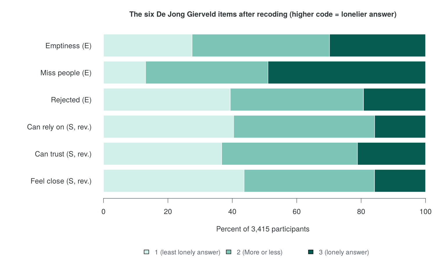
The published rule turns answers into a score
- Each item scores 1 for "More or less" or the lonely answer.
- The emotional and social subscales each run from 0 to 3.
- The total score runs from 0 (not lonely) to 6 (most lonely).
- Amira's scores match the supplied score for all 3,415 people.
Measurement error weakens correlations
Introduction and Overview
Many of the variables in health research describe things that cannot be observed directly. Loneliness, social support, depressive symptoms and health literacy are measured by asking people several questions and combining their answers into a score. The quality of every later analysis depends on that score. Lesson 2, Section 3 computed Cronbach's alpha, corrected item-total correlations and alpha-if-item-deleted, ran a parallel analysis and one-factor and two-factor exploratory factor analyses, and built prorated scores for depression and anxiety items that had no reverse-worded items. This lesson revisits those steps on the six De Jong Gierveld items, three of which are reverse-worded. This lesson takes the analyst's view of the same task: how scales are built, how their reliability and validity are judged, and how factor analysis and item response theory test whether the items behave as the scale's authors intended. This first section sets out the vocabulary of measurement, separates scales from indices, prepares and scores the loneliness items used throughout the lesson, and introduces classical test theory.
Learning Objectives
- Define constructs, latent variables, domains, items, indicators, instruments, scales, subscales and indices.
- Distinguish reflective measurement (a scale) from formative measurement (an index), and state why internal consistency applies only to the first.
- Describe levels of measurement, published scoring rules, cut-points and reverse-worded items.
- Recode, reverse-code and score the six items of the De Jong Gierveld Loneliness Scale in R.
- State the classical test theory model, define reliability, and explain how measurement error weakens a correlation.
Box 7.1 introduces the running case of the lesson, a manuscript on loneliness whose reviewer has raised two questions about how loneliness was measured.
Amira, a graduate student, has written a manuscript on loneliness using the 2021 wave of the Canadian Social Connection Survey (CSCS). She measured loneliness with the six-item De Jong Gierveld Loneliness Scale and added the six items into a single score. Her manuscript has returned with this comment from the second reviewer: "The authors add the six De Jong Gierveld items into a single score. Do the items measure one construct or two? The emotional subscale has three items. Is it reliable enough to analyze on its own?" Each section of this lesson adds one part of Amira's reply. Section 1 prepares and scores the items, Section 2 estimates their reliability, Section 3 assembles evidence of validity, and Section 4 tests the structure of the scale and drafts the revised Measures paragraph.
Answering either question requires precise terms for the parts of a measure, from the construct that a study sets out to measure to the score that enters the analysis. The first part of this section defines those terms.
The Vocabulary of Measurement
Measurement terms are often used loosely, and a reviewer will notice when a manuscript calls an index a scale or treats a single item as a construct. The terms below are used with these meanings throughout the course (Streiner, Norman & Cairney, 2015; DeVellis, 2017).
Figure 7.1 shows how the terms connect for the De Jong Gierveld Loneliness Scale, from the construct at the top, through its two domains and six items, to the instrument and scoring rule at the bottom. The six flip cards that follow the figure define each term and give an example of its use.
Two of these terms, scale and index, describe measures that both combine several items into one number. They differ in how the items relate to the construct, and the next part explains why that difference decides which statistics can be used to judge a measure.
Scales and Indices: Reflective and Formative Measurement
A scale and an index both combine several items into one number, yet they rest on different models of how the items relate to the construct (Bollen & Lennox, 1991; Diamantopoulos & Winklhofer, 2001). In reflective measurement, the construct causes the answers. A person who is lonely is more likely to report a sense of emptiness and more likely to report feeling rejected, so the answers to the items rise and fall together, and any one item could be replaced by a similar item without changing what is measured. In formative measurement, the components define the construct. A person is socially isolated because they are unmarried, rarely see family or friends and belong to no groups; isolation does not cause those circumstances. The components of an index can be unrelated to each other, and removing one changes the meaning of the index.
Figure 7.2 draws the two models side by side. The three tabs that follow it describe one reflective scale and two formative indices, and Box 7.2 explains why the distinction matters when a measure is analyzed.
The De Jong Gierveld Loneliness Scale (De Jong Gierveld & Van Tilburg, 2006) is reflective. Each item is a symptom of loneliness, so people who are lonelier are expected to give lonelier answers to every item. The items are interchangeable within a domain: "There are many people I can trust completely" and "There are enough people I feel close to" are two ways of asking about the same experience. Internal consistency, factor analysis and item response theory all assume this kind of model.
An area deprivation index, such as the Pampalon deprivation index used in Canadian health planning (Pampalon & Raymond, 2000), is formative. It combines census measures of education, employment and income with measures of household structure such as the share of people living alone. A neighbourhood is deprived because of these conditions, and the components need not move together: an area can have high employment and many people living alone. Each component is chosen because it is part of the definition, so dropping one changes what the index means.
The CSCS file contains the social isolation index of Steptoe and colleagues (2013), which gives one point each for being unmarried and not living with a partner, having less than monthly contact with children, with other family and with friends, and taking part in no groups or organizations. It is formative: a person who has no children is not thereby likely to belong to no clubs. Section 2 shows in R that these components barely correlate, which is expected for an index and is no evidence against it.
Box 7.2: Why the distinction matters for analysis
Internal consistency statistics such as Cronbach's alpha (Section 2) measure how strongly the items of a scale move together. For a reflective scale, high correlations among items are expected, and low correlations suggest a problem. For a formative index, low correlations among components are normal, so an alpha computed for an index says nothing about its quality. The validity of an index is judged by whether its components cover the definition of the construct and whether the index relates to other variables as theory predicts.
A reflective scale and a formative index are therefore judged by different evidence. Either kind of measure must first be scored, and the next part turns to the levels of measurement and the scoring rules on which scoring depends.
Levels of Measurement, Scoring Rules and Cut-points
Before the answers to several items are combined, the analyst needs to know what kind of values the answers are and how the authors of the scale intended them to be scored. Box 7.3 reviews the four levels of measurement and explains why each De Jong Gierveld item is treated as ordinal and a sum of items as approximately interval. The published scoring rule of the scale and the use of cut-points are described after the box.
Box 7.3: Background: Levels of measurement
Stevens (1946) described four levels of measurement. Nominal values are labels with no order, such as province of residence. Ordinal values have an order with unknown spacing, such as the answers "No", "More or less" and "Yes". Interval values have equal spacing without a true zero, such as temperature in degrees Celsius, and ratio values have equal spacing and a true zero, such as age or income. The level decides which summaries make sense: a mode for nominal values, a median for ordinal values, and means and differences for interval and ratio values.
Each De Jong Gierveld item is ordinal. A single Likert-type item is treated as ordinal because its few answers are ordered labels, and nothing shows that the steps from one answer to the next are equal. A sum of several ordinal items is usually treated as approximately interval: adding items spreads the scores over many values, and the uneven spacing of each item's answers tends to average out across items, so means and linear regression give sensible results. The convention works well when there are several items and the score takes many values, and it is weaker when a score has only a few possible values, as the subscales here do (0 to 3).
For optional reading, HSCI 207 Lesson 7, Section 3 introduces the four levels, and HSCI 230 Lesson 7, Section 1 ("The Problem of Scale Level") discusses when ordinal scores can be treated as interval.
A published scale comes with a scoring rule, and the rule should be followed exactly so that scores can be compared with other studies. The De Jong Gierveld rule is dichotomous: each item scores 1 if the answer is "More or less" or the lonely answer, and 0 otherwise (De Jong Gierveld & Van Tilburg, 2006). The three emotional items are added to give the emotional subscale (0 to 3), the three social items give the social subscale (0 to 3), and the two subscales are added to give the total (0 to 6). Some scales also publish a cut-point, a score at or above which a person is classified as having the condition. The CSCS file supplies a yes or no version of the total in which scores of 2 to 6 are classified as lonely. A cut-point converts a score into a category and discards information, so it should be taken from the scale's documentation, stated in the manuscript, and used only when the research question needs a category.
The published rule gives a point for an answer of "More or less" or for the lonely answer on each item, so the lonely answer must be identified for every item. For three of the six De Jong Gierveld items the lonely answer is "No", and these items must be recoded before they are combined, as the next part explains.
Reverse-Worded Items
Many scales mix negatively and positively worded items so that a respondent who agrees with every statement, a habit called acquiescence, does not receive an extreme score. The De Jong Gierveld scale does this. For the three emotional items ("I experience a general sense of emptiness", "I miss having people around me" and "I often feel rejected"), "Yes" is the lonely answer. For the three social items ("There are plenty of people I can rely on when I have problems", "There are many people I can trust completely" and "There are enough people I feel close to"), "No" is the lonely answer. Before the items can be combined, the positively worded items must be reverse-coded so that a higher number means a lonelier answer on every item.
Equation 7.1 gives the general rule for reversing the codes of an item, whatever the range of those codes.
Leaving a reverse-worded item unreversed is one of the most common errors in survey analysis. The item then counts in the wrong direction, the total score mixes loneliness with its opposite, and every statistic computed from it is distorted. Section 2 shows in R how much the reliability of the scale falls when this step is skipped. A cross-tabulation of the original and reversed codes, as in Activity 7.1, is a quick check that the reversal worked.
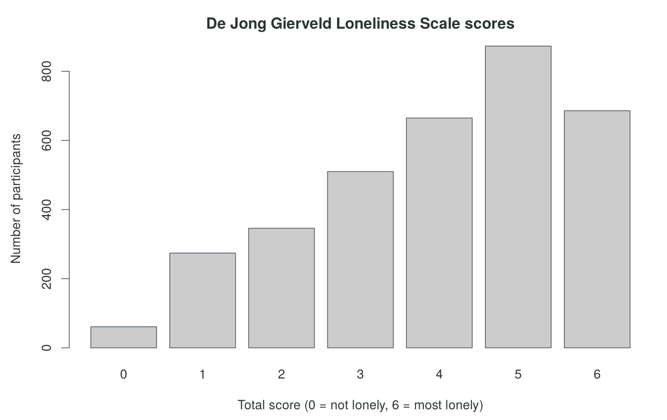
The two R activities that close this part prepare the data used throughout the lesson. Activity 7.1 loads the 2021 wave of the CSCS, converts the text answers of the six items to numbers, applies Equation 7.1 to the three social items and checks each step with a cross-tabulation. Activity 7.2 applies the published scoring rule to form the two subscale scores and the total score, checks the total against the score supplied with the CSCS file, and draws the bar chart of total scores shown in Figure 7.3.
This activity loads the 2021 wave of the Canadian Social Connection Survey and prepares the six De Jong Gierveld items exactly as the Factor Analysis and Scale Scoring walkthrough does, so every number in this lesson matches the walkthrough. The file is read directly from GitHub, so an internet connection is needed. Open a new R script, paste each block in turn and run it.
github_url <- "https://raw.githubusercontent.com/jorgeandr3s/heal/main/cscs/public_data/CSCS2025_full_cleaned_deidentified_data_and_metadata.RData"
load(url(github_url))     # loads a data frame called data
dim(data)                 # rows (survey responses) and columns

# Keep the 2021 wave, which gives one row per person
data <- data[data$SURVEY_collection_year == 2021, ]
dim(data)The full file has 13,219 rows across several survey years. Keeping the 2021 wave leaves 4,045 people, one row per person, with the same 3,247 columns.
# A small data frame with short names for the six items
dj <- data.frame(
  emptiness = data$LONELY_dejong_emotional_social_loneliness_scale_emptiness,
  miss      = data$LONELY_dejong_emotional_social_loneliness_scale_miss,
  rejected  = data$LONELY_dejong_emotional_social_loneliness_scale_rejected,
  rely      = data$LONELY_dejong_emotional_social_loneliness_scale_rely,
  trust     = data$LONELY_dejong_emotional_social_loneliness_scale_trust,
  close     = data$LONELY_dejong_emotional_social_loneliness_scale_close)

# The answers are stored as text categories
table(dj$emptiness, useNA = "ifany")
table(dj$rely, useNA = "ifany")The answers are stored as text. Besides "Yes", "More or less" and "No", there are 27 people who saw the emptiness item without answering it ("Presented but no response") and 536 who were not shown it (NA). The order in which the categories print is the order in the file and has no meaning.
# Text to numbers: No = 1, More or less = 2, Yes = 3
# Anything else ("Presented but no response" or NA) stays NA
dj$emptiness_n <- NA
dj$emptiness_n[dj$emptiness == "No"] <- 1
dj$emptiness_n[dj$emptiness == "More or less"] <- 2
dj$emptiness_n[dj$emptiness == "Yes"] <- 3

dj$miss_n <- NA
dj$miss_n[dj$miss == "No"] <- 1
dj$miss_n[dj$miss == "More or less"] <- 2
dj$miss_n[dj$miss == "Yes"] <- 3

dj$rejected_n <- NA
dj$rejected_n[dj$rejected == "No"] <- 1
dj$rejected_n[dj$rejected == "More or less"] <- 2
dj$rejected_n[dj$rejected == "Yes"] <- 3

dj$rely_n <- NA
dj$rely_n[dj$rely == "No"] <- 1
dj$rely_n[dj$rely == "More or less"] <- 2
dj$rely_n[dj$rely == "Yes"] <- 3

dj$trust_n <- NA
dj$trust_n[dj$trust == "No"] <- 1
dj$trust_n[dj$trust == "More or less"] <- 2
dj$trust_n[dj$trust == "Yes"] <- 3

dj$close_n <- NA
dj$close_n[dj$close == "No"] <- 1
dj$close_n[dj$close == "More or less"] <- 2
dj$close_n[dj$close == "Yes"] <- 3

# Check: each answer should map to one number
table(dj$emptiness, dj$emptiness_n, useNA = "ifany")The cross-tabulation is the check. Every "No" became 1, every "More or less" became 2 and every "Yes" became 3, and both kinds of missing answer became NA. The same pattern of code is repeated for the other five items.
# Reverse-code the three positively worded items: for these
# items "No" (1) is the lonely answer. Subtracting from 4 flips
# the scale: 1 becomes 3, 2 stays 2, and 3 becomes 1.
dj$rely_r  <- 4 - dj$rely_n
dj$trust_r <- 4 - dj$trust_n
dj$close_r <- 4 - dj$close_n
table(dj$rely_n, dj$rely_r) # check: 1 -> 3, 2 -> 2, 3 -> 1The table confirms the reversal for the "rely" item: the 546 people coded 1 ("No", the lonely answer) now have a 3, and the 1,409 people coded 3 ("Yes") now have a 1. The 1,526 "More or less" answers stay at 2.
# One data frame of six items, higher = lonelier
items <- data.frame(emptiness = dj$emptiness_n,
                    miss      = dj$miss_n,
                    rejected  = dj$rejected_n,
                    rely      = dj$rely_r,
                    trust     = dj$trust_r,
                    close     = dj$close_r)
items <- na.omit(items)   # people who answered all six items
nrow(items)The items data frame holds the 3,415 people who answered all six items, with a higher code meaning a lonelier answer on every item. Sections 2 and 4 analyze this data frame.
R Reflect on what you just ran
Use the questions below to interpret the output you produced. Look at your console output before answering.
1. Why must the rely, trust and close items be reverse-coded before the six items are combined, and how does the table from table(dj$rely_n, dj$rely_r) show that the reversal worked?
2. How many people are in the 2021 wave, how many answered all six items, and what happened to people who saw an item but gave no answer?
items data frame keeps the 3,415 who answered all six items. People coded "Presented but no response" were left as NA by the recoding, because only "No", "More or less" and "Yes" were assigned numbers, and na.omit() then removed anyone with an NA on any of the six items.3. What level of measurement is each recoded item, and what assumption is made when the codes 1, 2 and 3 are later added or averaged?
This activity continues from the one above and uses the dj data frame created there. It applies the published dichotomous scoring rule, forms the two subscale scores and the total score, and checks the total against the score supplied with the CSCS file.
# The published scoring rule: an item scores 1 for "More or
# less" or the lonely answer (a code of 2 or 3), and 0 otherwise.
dj$emptiness_01 <- as.numeric(dj$emptiness_n >= 2)
dj$miss_01      <- as.numeric(dj$miss_n >= 2)
dj$rejected_01  <- as.numeric(dj$rejected_n >= 2)
dj$rely_01      <- as.numeric(dj$rely_r >= 2)
dj$trust_01     <- as.numeric(dj$trust_r >= 2)
dj$close_01     <- as.numeric(dj$close_r >= 2)

# Add the items: two subscales (0 to 3) and a total (0 to 6)
dj$emotional_score <- dj$emptiness_01 + dj$miss_01 + dj$rejected_01
dj$social_score    <- dj$rely_01 + dj$trust_01 + dj$close_01
dj$total_score     <- dj$emotional_score + dj$social_score
table(dj$total_score, useNA = "ifany")A comparison such as dj$emptiness_n >= 2 gives TRUE or FALSE, and as.numeric() turns TRUE into 1 and FALSE into 0. The table shows the total score for the 3,415 people with complete answers; the 630 people with any missing item have no total. Scores pile up toward the top of the range: 873 people score 5 and 686 score 6.
# Check against the score supplied with the CSCS data
table(dj$total_score == data$LONELY_dejong_emotional_social_loneliness_scale_score,
      useNA = "ifany")

# Plot the total score
barplot(table(dj$total_score),
        main = "De Jong Gierveld Loneliness Scale scores",
        xlab = "Total score (0 = not lonely, 6 = most lonely)",
ylab = "Number of participants", col = "grey80")All 3,415 totals equal the score supplied with the data, and the 630 NA values are the same people in both versions. Agreement with a supplied score is a useful check whenever a data team has already scored a scale.
R Reflect on what you just ran
Use the questions below to interpret the output you produced. Look at your console output and plots before answering.
1. Under the published rule, which answers score 1 on the item "There are enough people I feel close to", and which code on dj$close_r do they correspond to?
close_r = 3 and "More or less" has close_r = 2, which is why the code uses dj$close_r >= 2.2. The CSCS file classifies total scores of 2 to 6 as lonely. Using the table of total scores, how many of the 3,415 people would be classified as lonely, and what information does the classification discard?
3. Why is it useful to compare your total score with LONELY_dejong_emotional_social_loneliness_scale_score before analyzing it?
The six items are now coded in the same direction and scored by the published rule, and the totals match the score supplied with the data. Figure 7.3 shows that the total scores are skewed toward the lonely end of the scale. Even a correctly prepared score contains some error, and the next part introduces the model that classical test theory uses to describe it.
Classical Test Theory
Classical test theory, set out formally by Lord and Novick (1968), is the simplest model of what an observed score contains. It states that each person's observed score X is the sum of a true score T and a random error E. The true score is the average score the person would obtain over many hypothetical repetitions of the measurement under the same conditions. The error is everything else: a question misread, a passing mood, a guess between two answers. The model assumes that errors average zero, that they are unrelated to the true score, and that the errors of different measurements are unrelated to each other.
Equation 7.2 states the model and the definition of reliability that follows from it.
Reliability is therefore a property of scores in a population, and it depends on how much people in that population differ. The same scale can have higher reliability in a population with a wide range of loneliness than in a population in which almost everyone is equally lonely, because the true-score variance is larger in the first. For this reason a manuscript reports the reliability observed in its own sample as well as the value from the scale's original publication.
Measurement error weakens associations
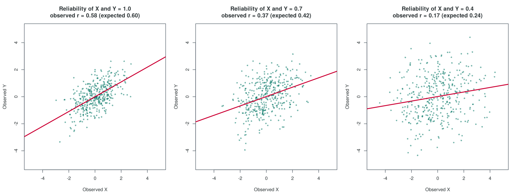
Random measurement error has a predictable effect on correlations. Spearman (1904) showed that when two variables are measured with error, the correlation between the observed scores is smaller than the correlation between the true scores, a result called attenuation.
Equation 7.3 gives Spearman's formula for the size of this effect and applies it to one set of values.
The corresponding result for a regression slope is simpler. When the exposure is measured with random error, the observed slope equals the true slope multiplied by the reliability of the exposure, a factor called the regression dilution ratio. With an exposure reliability of 0.60, a true slope of 2.0 is observed as about 1.2. Random error in the outcome leaves the slope unbiased and widens its confidence interval. For optional reading, HSCI 230 Lesson 7, Section 1 and HSCI 230 Lesson 9, Section 3 discuss attenuation and regression dilution.
The simulation in Interactive 7.1 generates 250 people whose true loneliness and true depressive symptoms have a chosen correlation, then adds random error to each measure. Lowering the reliability of either measure spreads the cloud of points and pulls the observed correlation toward zero. The panel also reports the correlation expected from Equation 7.3, so that the simulated and expected values can be compared.
📊 Interactive 7.1: Simulation: watch a correlation weaken as measurement error grows
The same weakening applies to the associations in Amira's manuscript. Box 7.4 returns to the running case and shows why the reliability of the emotional subscale matters for her results.
Amira's manuscript reports a correlation between loneliness and depressive symptoms. If the emotional subscale has a reliability of about 0.5, as Section 2 will show, then even a strong true association with a perfectly measured outcome would appear in her data at about √0.5 = 0.71 of its true size. A weak or null finding for the emotional subscale could therefore reflect the measure as much as the world. This is the practical reason that the reliability of each subscale must be reported, and that a low value must be discussed when the subscale is analyzed on its own.
This section has defined the parts of a measure, separated reflective scales from formative indices, prepared and scored the six De Jong Gierveld items, and introduced the classical test theory model, in which reliability is the proportion of observed-score variance that is true-score variance. Because true scores are never observed, reliability has to be estimated from data, which is the task of Section 2. The knowledge check and reflection that follow review the material of this section.
1. In the De Jong Gierveld Loneliness Scale, "emotional loneliness" and "social loneliness" are best described as:
2. A researcher builds a household food insecurity measure by adding points for low income, no vehicle and distance to a grocery store. Which description fits this measure?
3. An item is scored 1 to 5 and is worded positively, so 1 is the unhealthy answer. Which formula reverse-codes it so that a higher number is less healthy?
4. Under classical test theory, a scale has a reliability of 0.80. Which statement is correct?
5. Loneliness and depressive symptoms have a true correlation of 0.50. Both are measured with a reliability of 0.64. What observed correlation is expected?
✎ Reflection
This section distinguished reflective scales, in which a latent construct causes the answers to the items (so the items are expected to correlate), from formative indices, in which the components define the construct (so the components need not correlate). It also introduced classical test theory, in which an observed score equals a true score plus random error, reliability is the proportion of observed-score variance that is true-score variance, and Spearman's formula states that the observed correlation equals the true correlation multiplied by the square root of the product of the two reliabilities. Choose one multi-item measure used in health research, or use the six-item De Jong Gierveld Loneliness Scale (three emotional items and three social items, answered yes, more or less, or no). State whether it is a scale or an index and explain why, name any reverse-worded items and how you would recode them, and explain what a reliability of 0.60 for this measure would do to an observed correlation between it and an outcome.
Reliability
Introduction and Overview
Section 1 defined reliability as the proportion of the variance in observed scores that is true-score variance. This definition cannot be applied directly, because true scores are never observed. Reliability is therefore estimated from the consistency of a measurement: across two occasions, across two raters, or across the items of a scale. This section describes these kinds of reliability, explains why a single survey supports only one of them, and then teaches the most widely reported reliability statistic, Cronbach's alpha, together with its assumptions, its limits and its main alternative, McDonald's omega. It answers the second question in the reviewer's comment: whether the emotional subscale of the De Jong Gierveld scale is reliable enough to analyze on its own.
Learning Objectives
- Compare test-retest, inter-rater and internal consistency reliability, and state which can be estimated from a single cross-sectional survey.
- Compute and interpret an intraclass correlation for test-retest reliability and Cohen's kappa for agreement between two raters.
- Compute Cronbach's alpha, corrected item-total correlations and alpha-if-item-deleted with
psych::alpha(), and interpret each part of the output. - Explain the assumptions and limits of alpha, including why a high alpha does not show that a scale is unidimensional.
- Compute McDonald's omega from a one-factor model and explain when it differs from alpha.
- Show how failing to reverse-code items lowers alpha, and explain why internal consistency does not apply to an index.
The section begins with the three kinds of reliability and the study design that each one requires, because the design of the CSCS limits which of them Amira can estimate.
Three Kinds of Reliability
Every reliability statistic measures consistency, and the kinds of reliability differ in what the consistency is across. The choice is driven by the main source of error in the measurement: the occasion on which it is made, the person who makes it, or the particular items used.
Table 7.1 sets out the three kinds of reliability, the question each one answers, the design it needs and the statistic usually reported.
Table 7.1. Three kinds of reliability, with the design and the usual statistic for each.
| Kind of reliability | Question it answers | Design needed | Usual statistic |
|---|---|---|---|
| Test-retest | Do the same people get similar scores on two occasions? | The measure is given twice, with an interval short enough that the construct has not changed (often one to four weeks). | Intraclass correlation coefficient (ICC) for scores; kappa for categories |
| Inter-rater | Do two observers give the same rating to the same person? | Two or more raters assess the same people independently. | Cohen's kappa for categories; ICC for scores |
| Internal consistency | Do the items of one scale move together on one occasion? | One administration of a multi-item scale. | Cronbach's alpha; McDonald's omega |
Test-retest reliability for a continuous score is usually summarized with an intraclass correlation coefficient, which measures agreement as well as correlation. A Pearson correlation between two occasions can be high even if everyone scored five points higher the second time, whereas the intraclass correlation penalizes such a shift. Worked Example 7.1 shows the difference. It applies Equation 7.4, the intraclass correlation for absolute agreement, to hypothetical scores for six people measured on two occasions, and then repeats the calculation after a uniform shift in the second set of scores.
Worked Example 7.1: A test-retest intraclass correlation
Six people complete a symptom scale scored 0 to 20 on two occasions two weeks apart (hypothetical data). The intraclass correlation for absolute agreement compares the variation between people with the variation that remains: the disagreement between occasions for the same person, and any systematic shift from one occasion to the other.
| Person | A | B | C | D | E | F |
|---|---|---|---|---|---|---|
| Occasion 1 | 4 | 7 | 9 | 12 | 14 | 17 |
| Occasion 2 | 5 | 6 | 10 | 11 | 15 | 16 |
For these data, MSR = 42.4, MSC = 0 (both occasions have a mean of 10.5) and MSE = 0.6, so ICC = (42.4 − 0.6) ÷ (42.4 + 0.6 − 0.2) = 41.8 ÷ 42.8 = 0.98. The Pearson correlation is 0.97. Now suppose that every person scores 4 points higher on the second occasion. The Pearson correlation is unchanged at 0.97, because it ignores a shift that is the same for everyone. MSC rises to 48.0, and the ICC falls to 41.8 ÷ (43.0 + 15.8) = 0.71, because people no longer receive the same score twice.
Koo and Li (2016) suggest reading an ICC below 0.50 as poor reliability, 0.50 to 0.75 as moderate, 0.75 to 0.90 as good and above 0.90 as excellent, preferably judged from its 95% confidence interval. The first version of the table shows excellent test-retest reliability and the shifted version moderate reliability. This intraclass correlation coefficient is a different application of the same kind of variance ratio as the intracluster correlation coefficient used for clustered data in Lesson 5: there the clusters are clinics or people measured repeatedly, and here the repeated measurements of each person are the subject of interest.
Inter-rater reliability for categories, the second row of Table 7.1, is usually summarized with Cohen's kappa. Box 7.5 gives its formula as Equation 7.5 and works through two examples, the second of which shows how a rare category lowers kappa.
Box 7.5: Background: Cohen's kappa for agreement on categories
When two raters classify the same people into categories, the proportion of people on whom they agree (the observed agreement, po) overstates their reliability, because some agreement would occur by chance. Cohen's kappa corrects for this. The expected chance agreement, pe, is calculated from each rater's own proportions in each category.
Suppose two interviewers each classify the same 100 participants as lonely or not lonely. Both say lonely for 20 and not lonely for 65, so po = 0.85. The first interviewer calls 30% of participants lonely and the second 25%, so pe = 0.30 × 0.25 + 0.70 × 0.75 = 0.60, and κ = (0.85 − 0.60) ÷ (1 − 0.60) = 0.63. A rare category lowers kappa, because chance agreement on the common category is then high. If only 6% of participants are called lonely by each interviewer and they agree on 92 of 100, pe = 0.06 × 0.06 + 0.94 × 0.94 = 0.887 and κ = (0.92 − 0.887) ÷ (1 − 0.887) = 0.29, although agreement looks high.
For fuller treatments (optional reading), see HSCI 341 Lesson 5, Section 1, and HSCI 241 Lesson 7, Section 3.5.
Box 7.6 applies Table 7.1 to the CSCS and identifies the kinds of reliability that Amira can estimate from her data.
Box 7.6: What the CSCS can and cannot show
The 2021 wave of the CSCS asked the loneliness items once, in a self-completed online questionnaire with no interviewer or rater. Amira can therefore estimate internal consistency in her own sample, but she cannot estimate test-retest or inter-rater reliability. Evidence on the stability of the De Jong Gierveld scale over time has to come from the published literature on the scale, and her Measures paragraph should cite it as such and make clear which statistics were computed in her sample.
Internal consistency is therefore the only kind of reliability that Amira can estimate from the CSCS. The next part introduces the statistic most often used to estimate it, Cronbach's alpha.
Cronbach's Alpha
Cronbach's alpha is the most widely reported estimate of internal consistency, and the course has used it once already. Box 7.7 recalls that analysis from Lesson 2 and poses a retrieval question, which the standardized form of the formula in this part answers.
Box 7.7: Recall: Lesson 2, Section 3 (Building Scales)
The R activity in Lesson 2, Section 3 computed Cronbach's alpha for the seven depression items of the course dataset (alpha = 0.904), together with the alpha-if-item-deleted values and the corrected item-total correlations (r.drop, from 0.65 to 0.74). Every alpha-if-item-deleted value was below 0.904, so every item contributed. This section adds the formula behind alpha, its standardized form and McDonald's omega, and applies them to the De Jong Gierveld items.
Retrieval question. Why does alpha rise when items are added to a scale, even when the new items correlate with the others no more strongly than the existing items do?
Cronbach (1951) introduced coefficient alpha as a lower bound to the reliability of a sum of items, and it remains the statistic that reviewers most often expect to see. Alpha compares the variances of the individual items with the variance of the total score. When the items move together, people who score high on one item tend to score high on the others, so the total varies much more than the items do separately and alpha approaches 1. When the items are unrelated, the variance of the total is close to the sum of the item variances and alpha approaches 0.
Equation 7.6 gives alpha in its raw form, computed from the variances of the items and of the total score, and in its standardized form, computed from the average correlation between pairs of items.
The standardized formula shows that alpha depends on two things: the number of items and the strength of their correlations. With an average correlation of 0.25, three items give an alpha of 0.50, but twelve items with the same average correlation would give 3 / 3.75 = 0.80. Short subscales therefore tend to have lower alphas than long scales, even when their items are of equal quality, which is part of the reason the three-item emotional subscale has a low value.
Several conventions are used to judge alpha. Nunnally (1978) suggested that about 0.70 suffices in the early stages of research, that about 0.80 is adequate for basic research, and that 0.90 or higher is needed when scores are used to make decisions about individuals, such as a clinical cut-point; the widely used minimum of 0.70 comes from the first of these. Very high values, above about 0.90 to 0.95, can indicate that some items are close paraphrases of each other, which adds length without adding information (Streiner, 2003). These conventions are guides for judgement, and a manuscript should report the value and its confidence interval and let readers judge it in context.
Activity 7.3 applies these ideas to the De Jong Gierveld items in R, and the rest of this section draws on its results.
This activity continues from the Section 1 activities and uses the items and dj data frames created there. Alpha and omega are therefore computed from the three-point item codes in items (1 to 3, after reverse-coding), whereas the subscale and total scores follow the published 0 or 1 rule. It needs the psych package. It computes alpha for each subscale, reads the item statistics, compares alpha for the six items with and without reverse-coding, computes omega for each subscale, and shows what alpha does with an index.
# install.packages("psych")   # run once, if not yet installed
library(psych)    # alpha() and omega()
emotional_items <- items[, c("emptiness", "miss", "rejected")]
social_items    <- items[, c("rely", "trust", "close")]
alpha(social_items)Reading the output. The first row gives raw_alpha 0.75 (computed from the item codes) and std.alpha 0.75 (computed from the correlations), with an average_r of 0.5. The Feldt 95% confidence interval runs from 0.74 to 0.77. Under Reliability if an item is dropped, removing any one item lowers alpha to 0.66 to 0.69, so every item contributes. Under Item statistics, r.drop is the corrected item-total correlation, the correlation of each item with the sum of the other two: 0.60, 0.59 and 0.56. The last table shows how often each answer was given.
round(alpha(emotional_items)$total, 2)               # overall alpha only
round(alpha(emotional_items)$alpha.drop[, 1:2], 2)   # alpha if each item is dropped
round(alpha(emotional_items)$item.stats[, "r.drop", drop = FALSE], 2) # item-totalThe $total, $alpha.drop and $item.stats parts of the result can be printed separately. For the emotional subscale, raw alpha is 0.51 with an average inter-item correlation of 0.25. Dropping miss would raise alpha to 0.64, whereas dropping either of the other items would lower it to about 0.2 to 0.3. The corrected item-total correlation for miss is 0.16, against 0.43 and 0.40 for the other two items.
# Alpha for all six items, correctly reverse-coded
round(alpha(items)$total[, 1:2], 2)

# What happens if we forget to reverse-code?
not_reversed <- data.frame(emptiness = dj$emptiness_n,
                           miss      = dj$miss_n,
                           rejected  = dj$rejected_n,
                           rely      = dj$rely_n,
                           trust     = dj$trust_n,
                           close     = dj$close_n)
round(alpha(na.omit(not_reversed))$total[, 1:2], 2)With the social items correctly reversed, alpha for all six items is 0.59. With the reversal skipped, it falls to 0.42. In both runs psych prints a note and then a warning that some items are negatively correlated with the first principal component. In the second run the flagged items are emptiness and rejected, because the unreversed social items now point the other way. In the first run the flagged item is miss, which is correctly coded but relates weakly, and slightly negatively, to the social items. The suggested option check.keys = TRUE would flip flagged items automatically, which in the first run would reverse a correctly coded item. Which items to reverse is decided by the scoring manual, and the warning is a prompt to check the coding.
# McDonald's omega from a one-factor model of each subscale
f_social <- fa(social_items, nfactors = 1)   # one-factor model
lambda <- f_social$loadings[, 1]             # the three loadings
round(lambda, 2)
sum(lambda)^2 / (sum(lambda)^2 + sum(f_social$uniquenesses))   # omega

f_emo <- fa(emotional_items, nfactors = 1)
lambda <- f_emo$loadings[, 1]
round(lambda, 2)
sum(lambda)^2 / (sum(lambda)^2 + sum(f_emo$uniquenesses))fa(..., nfactors = 1) fits a one-factor model and returns the loadings and the unique variances ($uniquenesses). The last line of each block applies the omega formula. For the social items, omega is 0.754, the same as alpha, because the three loadings are similar. For the emotional items, omega is 0.568, higher than the alpha of 0.51, because the loading of miss (0.20) is far below the others. The omega() function in psych gives the same values.
# An index: the Steptoe social isolation index (CSCS supplies 0/1 codes,
# where 1 = isolated on that component)
iso <- data.frame(unmarried = data$LONELY_steptoe_isolation_index_unmarried_num,
                  clubs     = data$LONELY_steptoe_isolation_index_clubs_num,
                  friends   = data$LONELY_steptoe_isolation_index_friends_num,
                  children  = data$LONELY_steptoe_isolation_index_kids_num,
                  family    = data$LONELY_steptoe_isolation_index_other_fam_num)
iso <- na.omit(iso)
round(cor(iso), 2)
round(alpha(iso)$total[, 1:2], 2) # shown only to explain why it is not reportedThe five components of the Steptoe social isolation index correlate only weakly (from −0.10 to 0.36), and alpha is 0.34 for the 3,430 people with all five components. For a formative index this is expected: being unmarried does not make a person more likely to have little contact with friends. The value is printed here only to show why it should not be reported as the reliability of an index.
R Reflect on what you just ran
Use the questions below to interpret the output you produced. Look at your console output before answering.
1. Report alpha for the social and emotional subscales with their 95% confidence intervals where printed, and state in one sentence whether each is adequate for comparing groups in research.
2. Using the $alpha.drop and r.drop output for the emotional subscale, identify the weakest item and explain why dropping it from the main analysis would still be questionable.
miss ("I miss having people around me"): its corrected item-total correlation is 0.16, against 0.43 and 0.40 for the other items, and alpha would rise from 0.51 to 0.64 without it. Dropping it would make the subscale differ from the published scoring rule, so the scores would not be comparable with other studies, and choosing items after seeing the data overstates reliability in new samples. It is better to keep the published subscale, report the weak item, and run a sensitivity analysis with the two-item version.3. Why is omega higher than alpha for the emotional subscale but equal to alpha for the social subscale?
Activity 7.3 gives an alpha of 0.75 for the social subscale and 0.51 for the emotional subscale, shows the six-item alpha falling from 0.59 to 0.42 when the reversal is skipped, and gives an alpha of 0.34 for an index whose components are not expected to correlate. Reading such values correctly requires knowing what alpha assumes, which the next part examines.
What Alpha Assumes and What It Cannot Show
Alpha is easy to compute and is often over-interpreted (Sijtsma, 2009; Dunn, Baguley & Brunsden, 2014). The accordion below sets out the five misconceptions that this lesson addresses, each with the evidence from the CSCS loneliness items.
The first item in the accordion also contains Box 7.8, which revisits a claim about alpha made in Lesson 2 and asks for it to be rewritten.
Alpha measures how strongly the items correlate on average, and a set of items can correlate on average even when they measure two or more constructs. Because alpha rises with the number of items, a long scale built from two distinct clusters can reach 0.80 or more. In the CSCS data the six De Jong Gierveld items have an alpha of 0.59, lower than the 0.75 of the three social items alone, because the emotional and social items correlate only weakly with each other. Whether a scale is unidimensional is a question for factor analysis (Section 4).
Box 7.8: Revisiting Lesson 2
Lesson 2, Section 3 stated: "An α of 0.904 indicates that the seven depression items measure essentially the same construct." Alpha shows how strongly the items correlate on average, which a set of items measuring two constructs can also do. The evidence in Lesson 2 that the depression items measure one construct came from its parallel analysis, which kept one factor, and from its one-factor solution, in which every loading was 0.69 or higher.
Question. Rewrite the Lesson 2 sentence so that it claims only what alpha shows.
Above about 0.95, a high alpha usually means that items repeat each other, for example "I feel lonely" and "I feel alone". Redundant items lengthen the questionnaire and burden respondents, and they can narrow the construct to whatever the repeated items share. A good scale covers the breadth of its construct, which keeps the item correlations moderate.
Alpha assumes a reflective model in which one construct causes all of the answers. The components of a formative index are not expected to correlate, so a low alpha for an index is expected and says nothing about its quality. Activity 7.3 shows that the components of the Steptoe social isolation index in the CSCS correlate between −0.10 and 0.36 and give an alpha of 0.34, a value that should not be reported as a measure of the index's reliability.
Reliability concerns random error, and validity concerns whether the score measures the intended construct. A bathroom scale that always reads three kilograms too heavy is perfectly consistent and systematically wrong. A loneliness scale could be highly reliable and still mainly measure general distress. Reliability limits validity, because a score that is mostly error cannot correlate strongly with anything, but it does not establish it. Section 3 takes up validity.
If positively and negatively worded items are summed as stored, half of the items count in the wrong direction. Activity 7.3 shows that the six-item alpha falls from 0.59 to 0.42 when the three social items are left unreversed. The total score would be distorted in the same way, and every association estimated with it would be biased toward zero.
Alpha also assumes that every item measures the construct equally well, a condition called tau-equivalence. Formally, each item is assumed to have the same loading on the common factor. When some items are stronger indicators than others, alpha underestimates the reliability of the total score. The assumption is plausible for the social items, whose loadings are similar, and clearly false for the emotional items, where one item is much weaker than the other two.
When the items differ in quality, a reliability coefficient that allows each item its own loading gives a better estimate of the reliability of the total score. The next part introduces such a coefficient, McDonald's omega.
McDonald's Omega
McDonald's omega (McDonald, 1999) estimates the reliability of a sum score from a factor model, which allows each item to have its own loading. For a scale with a single factor, omega is the share of the variance of the total score that is explained by the factor.
Equation 7.7 gives omega for a one-factor model and applies it to the loadings of the three social items.
When the loadings are equal, omega equals alpha, and when they differ, omega is the better estimate. The section's R activity computes omega for both subscales from a one-factor model fitted with fa(), which Section 4 explains in detail. The social loadings are similar (0.73, 0.73 and 0.67), and alpha and omega are both 0.75. The emotional loadings are very unequal (0.83, 0.20 and 0.58), so omega (0.57) is higher than alpha (0.51). Both values are low. Omega is now recommended alongside or in place of alpha in many fields, and reporting both lets readers compare a study with earlier work that reported only alpha.
Box 7.9 returns to the running case and applies these results to the weak emotional item identified in Activity 7.3.
The alpha output shows that the emotional item "I miss having people around me" has a corrected item-total correlation of 0.16, and that alpha for the emotional subscale would rise from 0.51 to 0.64 if it were dropped. It is tempting to delete the item and report the higher value. Amira decides against making that her main analysis, for three reasons. The published scoring rule uses all three items, so a two-item subscale would not be comparable with other studies of the scale. An alpha chosen after looking at the data overstates reliability in new samples. The item also covers a part of emotional loneliness (missing the presence of others) that the other two items do not. Her reply therefore keeps the published subscale as the main measure, reports alpha and omega for it, names the weak item, and adds a sensitivity analysis that repeats her main model with the two-item version. If the conclusions agree, the weak item has not driven them.
The card below links to a narrated R walkthrough of the same reliability analysis.
Narrated R walkthrough: Factor Analysis and Scale Scoring
The Factor Analysis and Scale Scoring walkthrough runs the same reliability analysis line by line with narration, from recoding the items to the effect of a missed reversal. It is a useful companion to Activity 7.3 for anyone who would like to see each step demonstrated before running it.
Open the Factor Analysis and Scale Scoring walkthroughThis section has shown that a single survey supports only internal consistency, that the social subscale of the De Jong Gierveld scale has adequate internal consistency (alpha and omega of 0.75), and that the emotional subscale has low internal consistency (alpha of 0.51 and omega of 0.57). It has also shown that alpha must be read with its assumptions in mind. A reliable score can still measure the wrong construct, so Section 3 turns to validity. The knowledge check and reflection that follow review the material of this section.
1. A study gives a fatigue questionnaire to the same patients twice, two weeks apart. Which kind of reliability does this design estimate?
2. Two subscales have the same average inter-item correlation of 0.30. One has 3 items and the other has 10. Which statement is correct?
3. A 20-item scale has alpha = 0.88. Which conclusion is justified?
4. For the emotional subscale, alpha is 0.51 and omega is 0.57. What best explains why omega is higher?
5. An analyst reports alpha = 0.34 for a five-component social isolation index. What is the main problem with this report?
✎ Reflection
Cronbach's alpha measures how strongly the items of a scale move together. It rises with the number of items and their average correlation, assumes that every item measures the construct equally well, and cannot show that a scale measures a single construct. McDonald's omega, computed from a one-factor model, allows the items to have different loadings. In the 2021 wave of the Canadian Social Connection Survey, the three-item social subscale of the De Jong Gierveld Loneliness Scale has alpha = 0.75 and omega = 0.75. The three-item emotional subscale has alpha = 0.51 and omega = 0.57. One emotional item, "I miss having people around me", has a corrected item-total correlation of 0.16, and alpha for the emotional subscale would rise to 0.64 without it. A reviewer has asked whether the emotional subscale is reliable enough to analyze on its own. Write the two to four sentences you would add to your reply to the reviewer, and explain in one further sentence why you would or would not drop the weak item from your main analysis.
Validity
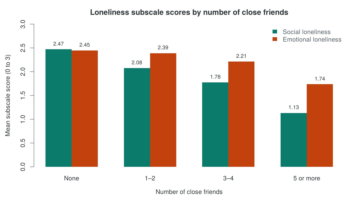
Scores fall as the number of close friends rises
Introduction and Overview
A reliable score is consistent, and consistency does not show that the score measures the intended construct. Validity concerns the meaning of scores: whether a loneliness score reflects loneliness or instead reflects low mood, social desirability or something else that the items happen to share. HSCI 230 Lesson 7 introduced construct validity and measurement error from the perspective of a reader appraising a study. HSCI 230 used construct validity for the broad question of whether an instrument captures its construct, which this lesson calls validity. This lesson reserves construct validity for evidence that scores relate to other measures as theory predicts (convergent, discriminant and known-groups evidence), and the COSMIN taxonomy later in the section groups structural and cross-cultural validity under construct validity. This section takes the analyst's perspective. It presents the kinds of validity evidence and the COSMIN taxonomy, frames validity as an argument for a particular use of scores in a particular population, and gathers construct validity evidence for the De Jong Gierveld scale from the CSCS data.
Learning Objectives
- Distinguish reliability from validity, and explain why a reliable measure is not necessarily valid.
- Describe content and face validity, criterion validity (concurrent and predictive), construct validity (convergent, discriminant and known groups) and structural validity.
- Explain validity as an argument assembled from several kinds of evidence for a particular use in a particular population.
- Use the COSMIN taxonomy to organize the measurement properties of an instrument.
- Define the minimal important difference and compare anchor-based and distribution-based estimates of it.
- Compute and interpret convergent, discriminant and known-groups evidence in R.
The section begins by setting reliability and validity side by side, and the parts that follow describe how evidence of validity is framed, classified and gathered.
Reliability and Validity
Reliability concerns random error, the scatter of scores around a person's true score. Validity concerns systematic error, whether the true score itself corresponds to the intended construct. The two are linked in one direction only. A score that is mostly random error cannot correlate strongly with anything, so low reliability limits validity. A highly reliable score can still measure the wrong construct, as a bathroom scale that always reads three kilograms heavy is consistent and wrong.
Figure 7.4 illustrates the relation with three dartboards, in which the spread of the darts stands for reliability and their position relative to the bullseye stands for validity.
A consistent score can therefore still miss its target, and validity has to be supported by evidence of its own. The next part describes how current measurement theory frames that evidence.
Validity as an Argument
Early textbooks listed "types of validity" as if a scale either had or lacked each one. Current measurement theory treats validity as a single, overall judgement about how well the evidence supports a particular interpretation and use of scores (Messick, 1989, 1995; AERA, APA & NCME, 2014). Kane (2013) describes validation as the construction of an argument in two steps. The first step states the interpretation and use: for example, "scores on the De Jong Gierveld scale rank adults in an online Canadian survey by their degree of loneliness, and differences in mean scores between groups reflect differences in loneliness". The second step gathers evidence for each claim that this interpretation depends on, including that the items cover loneliness, that the answers form the intended domains, that the scores relate to other variables as expected, and that the items work the same way in the groups being compared.
Two consequences follow. Support for a scale is always relative to a stated use in a stated population, so a scale cannot be called "valid" in general. Evidence that the De Jong Gierveld scale works well in the populations in which it was developed supports, without settling, its use with Canadian adults of all ages in an online survey. Validation is also cumulative: each study that uses a scale and reports how its scores behave adds to the argument.
Validity is therefore judged for a stated use in a stated population, and the next part describes the kinds of evidence from which the argument is assembled.
Kinds of Validity Evidence
Validity evidence is usually grouped into several kinds, each of which supports a different claim in the argument. The six flip cards below define content, face, criterion, convergent and discriminant, known-groups and structural evidence, and the paragraph after them explains which kinds carry most weight for a construct such as loneliness.
Criterion validity is the most direct evidence when a trusted gold standard exists, as it does for many diagnostic tests. For psychological constructs such as loneliness there is no gold standard, so the argument relies mainly on content, construct and structural evidence (Cronbach & Meehl, 1955). Construct validity is tested by writing down, before looking at the data, the correlations and group differences that theory predicts, and then checking them. COSMIN calls this hypothesis testing. Stating the hypotheses in advance guards against reading support into whatever pattern appears.
The next part presents the COSMIN taxonomy, which places these kinds of validity evidence alongside reliability and responsiveness.
The COSMIN Taxonomy
The COSMIN initiative (Consensus-based Standards for the selection of health Measurement Instruments) developed, through an international Delphi study, a taxonomy and definitions for the measurement properties of health instruments (Mokkink et al., 2010). It is widely used in systematic reviews of measurement instruments, and it is a useful checklist for the Measures paragraph of a manuscript.
Table 7.2 lists the three COSMIN domains with their measurement properties, the question that each property answers, and the evidence for the De Jong Gierveld scale that this lesson provides.
Table 7.2. The COSMIN domains and measurement properties, with the evidence for the De Jong Gierveld scale in this lesson.
| Domain | Measurement property | Question it answers | Evidence for the De Jong Gierveld scale in this lesson |
|---|---|---|---|
| Reliability | Internal consistency | Do the items of each domain move together? | Alpha and omega in the CSCS sample (Section 2) |
| Reliability | Are scores stable over occasions or raters? | Published studies only; not estimable from one CSCS wave | |
| Measurement error | How large is the error in a person's score? | Not assessed in this lesson | |
| Validity | Content validity (including face validity) | Do the items cover the construct? | Item wording based on Weiss's two domains (Section 1) |
| Construct validity: structural validity, hypothesis testing, cross-cultural validity | Do the items form the predicted domains, and do scores relate to other variables as predicted? | Factor analysis (Section 4); correlations and known groups (this section) | |
| Criterion validity | Do scores agree with a gold standard? | No gold standard for loneliness | |
| Responsiveness | Responsiveness | Do scores change when the construct changes? | Needs longitudinal data |
COSMIN also describes interpretability (for example, what size of difference in scores is meaningful) as an important characteristic of an instrument, alongside the three domains.
Interpreting change: the minimal important difference
Responsiveness asks whether scores change when the construct changes, and interpretability asks what a change of a given size means. The minimal important difference (MID) is the smallest change in scores that people would regard as important, or that would justify a change in care (Jaeschke, Singer & Guyatt, 1989). It is estimated in two ways. An anchor-based estimate links score changes to an external judgement, the anchor: for example, participants report at follow-up whether their loneliness is "a little better", and the MID is the mean change in score among those who chose that answer. A distribution-based estimate uses only the spread and the reliability of the scores. Two common versions are half a standard deviation of the baseline scores (Norman, Sloan & Wyrwich, 2003) and one standard error of measurement (Wyrwich, Tierney & Wolinsky, 1999).
Equation 7.8 defines the standard error of measurement used in the second distribution-based estimate.
Distribution-based values describe how large a change is compared with the spread of scores and the error in them, and they say nothing directly about importance, so anchor-based estimates are preferred when they exist and distribution-based values serve as a check. As an illustration, consider a loneliness scale scored 0 to 6 whose baseline scores have a standard deviation of 1.6 and a reliability of 0.75 (hypothetical values). Half a standard deviation is 0.8 points, and the SEM is 1.6 × √0.25 = 0.8 points; the two coincide whenever the reliability is 0.75. If participants who reported feeling "a little better" improved by 1.0 point on average, the anchor-based MID would be 1.0. A program that lowers the mean score by 0.4 points then produces a change below every estimate of the MID, even if a large trial finds it statistically significant.
Table 7.2 also shows that, beyond internal consistency, the CSCS data can add two kinds of validity evidence for the De Jong Gierveld scale: hypothesis testing through correlations and known groups, which the next part computes, and structural validity through factor analysis, which Section 4 tests.
Construct Validity Evidence from the CSCS
Before computing anything, Amira writes down what the theory of the scale predicts. Loneliness is usually defined as the distress that follows from a gap between the relationships a person has and those they want (Perlman & Peplau, 1981), and Weiss (1973) distinguished its emotional and social forms. The total score should therefore correlate positively with another loneliness measure, the three-item UCLA Loneliness Scale (Hughes et al., 2004), and negatively with perceived social support, measured in the CSCS with the Multidimensional Scale of Perceived Social Support (Zimet et al., 1988). It should correlate less strongly with anxiety symptoms (measured with the two-item GAD-2), a related but distinct construct. The social subscale, which concerns the wider network, should relate more strongly to social support and to the number of close friends than the emotional subscale does.
Activity 7.4 tests these predictions in the CSCS data, with a correlation matrix for the convergent and discriminant hypotheses and a comparison of subscale means by number of close friends for the known-groups hypothesis.
This activity continues from the Section 1 activities and uses the data and dj data frames, including the subscale and total scores created by the scoring activity. The other measures were scored by the CSCS team and are used as supplied: the three-item UCLA Loneliness Scale (3 to 9), the Multidimensional Scale of Perceived Social Support (an average from 1 to 7) and the two-item GAD-2 anxiety screener (0 to 6).
# Other measures in the CSCS file (already scored by the survey team)
val <- data.frame(total     = dj$total_score,
                  social    = dj$social_score,
                  emotional = dj$emotional_score,
                  ucla      = data$LONELY_ucla_loneliness_scale_score,
                  support   = data$PSYCH_zimet_multidimensional_social_support_scale_score,
                  anxiety   = data$WELLNESS_gad_score)
val <- na.omit(val)     # people with every score
nrow(val)
round(cor(val), 2) # correlations between every pair of measuresReading the matrix. The 3,053 people have every score. Read across the total, social and emotional rows. The convergent correlations for the total are 0.45 with the UCLA scale and −0.49 with social support (negative because more support goes with less loneliness), and the discriminant correlation with anxiety is lower at 0.33. The social subscale correlates −0.48 with support and 0.21 with anxiety. The emotional subscale correlates −0.26 with support and 0.32 with anxiety. The two subscales correlate 0.21 with each other.
# Known groups: people with no close friends should score higher
friends <- data$CONNECTION_social_num_close_friends_grouped
friends[friends == "Presented but no response"] <- NA
friends <- factor(friends, levels = c("None", "1–2", "3–4", "5 or more"))
round(tapply(dj$social_score, friends, mean, na.rm = TRUE), 2)
round(tapply(dj$emotional_score, friends, mean, na.rm = TRUE), 2)The first line gives the mean social subscale score (0 to 3) in each group, and the second gives the mean emotional subscale score. Social loneliness falls from 2.47 among people with no close friends to 1.13 among those with five or more. Emotional loneliness falls from 2.45 to 1.74. The grouping variable is set as a factor with its levels in order so that the groups print from fewest to most friends.
R Reflect on what you just ran
Use the questions below to interpret the output you produced. Look at your console output and plots before answering.
1. Before running the code, a theory-based hypothesis was stated: the social subscale should correlate more strongly with perceived social support than the emotional subscale does. Report the two correlations and state whether the hypothesis is supported.
2. Using the correlations for the total score, explain which values provide convergent evidence and which provide discriminant evidence, and whether the pattern is convincing.
3. Describe the known-groups result for the two subscales, and explain why the difference in the size of the two gradients fits Weiss's distinction between social and emotional loneliness.
The results support most of these predictions. The total score correlates 0.45 with the UCLA scale and −0.49 with perceived social support, and only 0.33 with anxiety, so the convergent correlations exceed the discriminant one. The gap is modest, which is common for constructs that share an emotional component. The two subscales show the distinct patterns the theory predicts: the social subscale relates most strongly to social support (−0.48, compared with −0.26 for the emotional subscale), whereas the emotional subscale relates more strongly to the UCLA scale and to anxiety. The known-groups comparison shows a steady gradient by number of close friends, much steeper for social loneliness (2.47 to 1.13) than for emotional loneliness (2.45 to 1.74). The two subscales correlate only 0.21 with each other.
Figure 7.5 plots the known-groups comparison for the two subscales. Box 7.10 then sets out two reasons for caution in reading these validity correlations.
Box 7.10: Interpreting validity correlations with care
Validity correlations are themselves attenuated by unreliability (Section 1). The emotional subscale has an alpha of 0.51, so its correlations with other measures are weakened, and part of the difference between the subscales' correlations could reflect their different reliabilities. The CSCS is also a cross-sectional online survey that recruited volunteers, so these correlations describe this sample and support, without proving, the same pattern in other populations.
Figure 7.5 compares mean scores between groups, and any such comparison rests on an assumption that the next part examines.
Measurement Invariance
A comparison of mean scores between groups, such as older and younger adults, assumes that the items relate to the construct in the same way in each group. If younger adults interpret "I miss having people around me" differently from older adults, a difference in mean scores could arise from the item's wording. Measurement invariance testing, introduced in HSCI 230 Lesson 7, checks this assumption by fitting the confirmatory factor model of Section 4 in each group and testing whether the loadings and item intercepts are equal. A full treatment is beyond this lesson. In a manuscript that compares groups, it is good practice to cite any published invariance evidence and to note comparisons for which it is missing.
With the kinds of evidence, the COSMIN headings and the CSCS results in place, the last part of this section shows how they are assembled into a validity argument for a Measures paragraph.
Assembling the Validity Evidence for a CSCS Measure
A Measures paragraph for a CSCS measure needs a short validity argument. The task in Box 7.11 sets out how to assemble one. It draws on the measure's published sources and on the analysis of the CSCS data.
Choose one multi-item measure in the CSCS (for example, the De Jong Gierveld scale, the three-item UCLA Loneliness Scale, the Multidimensional Scale of Perceived Social Support, the PHQ-2 or the GAD-2). First, state the interpretation and use in one sentence, naming the population. Second, find the scale's original development paper and, if one exists, a validation study in a population like the CSCS sample, and note the evidence each provides under the COSMIN headings (content, structural, hypothesis testing, criterion, reliability). Third, note what an analysis of the CSCS data adds: internal consistency in the study sample, and one or two pre-stated correlations or group differences. Fourth, record what is missing, such as test-retest evidence or measurement invariance across the groups being compared. The result is a table of four rows that becomes two or three sentences of a Measures paragraph like the one drafted in Section 4.
This section has treated validity as an argument for a particular use of scores in a particular population, organized the evidence for it with the COSMIN taxonomy, and gathered construct validity evidence for the De Jong Gierveld scale from the CSCS. Structural validity, the evidence that the reviewer's first question calls for, requires a latent variable model, and Section 4 introduces the models used to test it. The knowledge check and reflection that follow review the material of this section.
1. A bathroom scale always reads exactly 2 kg heavier than the true weight. How is this measure best described?
2. A new depression screener is compared with a structured clinical interview carried out on the same day. Which kind of evidence does this provide?
3. In the CSCS, the De Jong Gierveld total correlates 0.45 with the UCLA Loneliness Scale and 0.33 with anxiety symptoms. Which interpretation is best?
4. Which statement reflects the current view of validity described by Messick and Kane?
5. In the COSMIN taxonomy, factor analysis that tests whether items form the predicted domains provides evidence for which measurement property?
6. A loneliness scale has a baseline standard deviation of 2.0 and a reliability of 0.84. A program lowers the mean score by 0.6 points. Using one standard error of measurement (SEM) as the distribution-based minimal important difference, does the change exceed it?
✎ Reflection
Validity is argued for a stated use of scores in a stated population, from several kinds of evidence: content and face validity (the items cover the construct), criterion validity (agreement with a gold standard, concurrent or predictive), construct validity (convergent evidence from strong correlations with measures of the same construct, discriminant evidence from weaker correlations with related but distinct constructs, and known-groups differences), and structural validity (the items form the predicted domains). In the 2021 Canadian Social Connection Survey, the De Jong Gierveld loneliness total correlates 0.45 with the three-item UCLA Loneliness Scale, −0.49 with perceived social support and 0.33 with anxiety symptoms. The social subscale correlates −0.48 with social support and the emotional subscale −0.26. Mean social loneliness (0 to 3) falls from 2.47 among people with no close friends to 1.13 among those with five or more, while mean emotional loneliness falls from 2.45 to 1.74. No gold standard for loneliness exists. Write a short validity argument (four to six sentences) for using the De Jong Gierveld scale to compare levels of loneliness between groups of Canadian adults in an online survey. State the intended use, cite at least three kinds of evidence from those listed, and name one piece of evidence that is missing.
Latent Variable Models: Factor Analysis and Item Response Theory
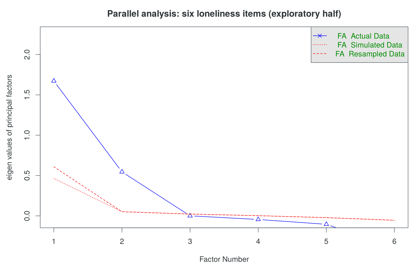
Parallel analysis suggests two factors
- The overall KMO is 0.68, which is adequate.
- Parallel analysis keeps two factors.
- Oblimin rotation allows the factors to correlate (r = 0.29).
- The miss item loads below 0.3 on both factors.
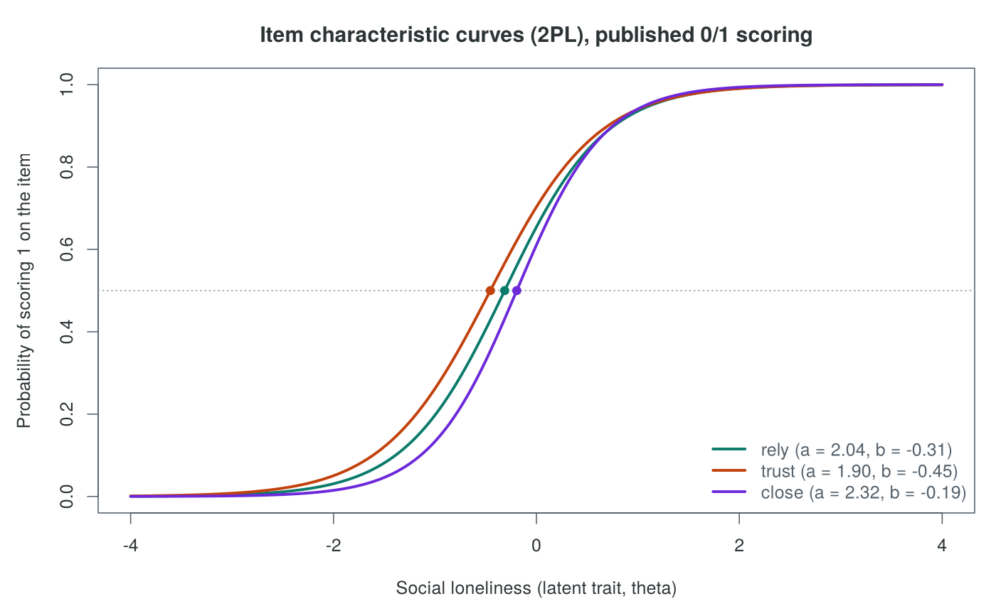
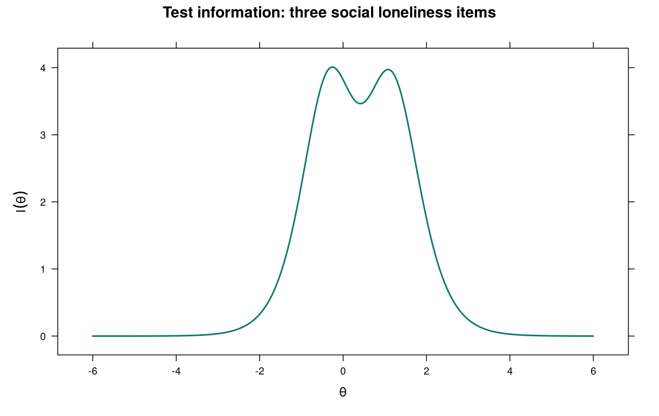
Where on the trait do the items measure well?
Introduction and Overview
Sections 2 and 3 produced two hints that the six De Jong Gierveld items do not form a single construct: the six-item alpha (0.59) is lower than the alpha of the social subscale alone (0.75), and the two subscales correlate only 0.21 and relate differently to other measures. A latent variable model can test this directly. This section teaches exploratory factor analysis (EFA), which lets the data suggest a structure, and confirmatory factor analysis (CFA), which tests a structure stated in advance. It then introduces item response theory (IRT) at a conceptual level, using curves estimated from the loneliness items, and compares it with classical test theory. The section ends with the Measures paragraph of Amira's revised manuscript. Lesson 8 extends the confirmatory model of this section into structural equation models.
Learning Objectives
- Describe the common factor model and interpret a standardized loading.
- Carry out an exploratory factor analysis in R: check factorability with the KMO and Bartlett tests, choose the number of factors with parallel analysis, apply an oblique rotation and read a loading matrix.
- Specify and fit a confirmatory factor analysis in lavaan, and compare one-factor and two-factor models with the CFI, TLI, RMSEA and SRMR.
- Explain item difficulty, item discrimination, item characteristic curves and test information, and distinguish the Rasch, two-parameter and graded response models.
- Compare item response theory with classical test theory, and report the structure and reliability of a scale in a Measures paragraph.
- Describe latent class analysis as a latent variable model for a categorical latent variable, and explain how the number of classes is chosen.
The first part presents the common factor model on which both exploratory and confirmatory factor analysis rest.
The Common Factor Model
A factor model treats the answer to each item as the sum of two parts: a part caused by a latent factor that the items share, and a unique part that belongs to the item alone (Spearman, 1904; Thurstone, 1947). The loading λ describes how strongly the item depends on the factor. When the items and the factor are standardized, the loading is the correlation between the item and the factor, and its square is the share of the item's variance that the factor explains, called the communality. The rest is the unique variance, which includes measurement error and anything specific to the item's wording.
Equation 7.9 writes the model for one standardized item.
Figure 7.6 draws the two-factor model of the De Jong Gierveld scale, with the standardized loadings and the factor correlation from the confirmatory model fitted later in this section.
Factor analysis and the reliability statistics of Section 2 rest on the same reflective model, so they answer related questions. Alpha and omega summarize how well a set of items measures whatever they share, assuming there is one thing they share. Factor analysis asks how many things they share and which items measure each one.
A factor model can be used to find out how many factors a set of items share or to test a structure stated in advance. The next part describes both uses and the order in which Amira applies them.
Exploratory and Confirmatory Factor Analysis
Exploratory factor analysis lets every item load on every factor and estimates the loadings from the data. It is used when the structure is unknown, for example when a new scale is being developed, and it suggests how many factors there are and which items belong together. Confirmatory factor analysis tests a structure stated in advance: each item loads only on the factor the theory assigns it to, and all other loadings are fixed at zero. A confirmatory model can be rejected by the data, which makes it the stronger test of a published scale's structure.
Exploring and confirming in the same data would let the confirmatory model reward whatever the exploration happened to find. Amira therefore splits the 3,415 participants at random into two halves of 1,708 and 1,707, explores in the first and confirms in the second. The split uses set.seed(2021) so that it is the same every time the code is run, and it matches the split in the Factor Analysis and Scale Scoring walkthrough.
Exploratory factor analysis in four steps
An exploratory factor analysis proceeds in four steps, set out in the accordion below: checking that the items are suitable, choosing the number of factors, rotating the solution and reading the loading matrix. Step 2 includes the parallel analysis plot for the exploratory half as Figure 7.7, and Step 3 includes Box 7.12, which revisits the rotation used in Lesson 2.
Factor analysis needs items that correlate. The Kaiser-Meyer-Olkin (KMO) measure of sampling adequacy compares the correlations between items with their partial correlations. Kaiser (1974) labelled values of 0.90 or above "marvelous", values in the 0.80s "meritorious", the 0.70s "middling", the 0.60s "mediocre", the 0.50s "miserable" and values below 0.50 "unacceptable", and about 0.6 is often treated as a practical minimum. Bartlett's test of sphericity tests whether the correlation matrix differs from one in which all correlations are zero; with samples of this size it is almost always significant, so it is a minimal check. For the exploratory half, the overall KMO is 0.68 and Bartlett's test gives a chi-square of 1,912 on 15 degrees of freedom (p < 0.001).
Each factor has an eigenvalue that describes how much of the items' variance it explains. The old rule of keeping every factor with an eigenvalue above 1 (the Kaiser criterion) often keeps too many factors. Parallel analysis (Horn, 1965) compares each eigenvalue from the data with the eigenvalues obtained from random data of the same size, and keeps the factors whose eigenvalues exceed the random ones. For the loneliness items, two eigenvalues lie above the random line, and fa.parallel() reports that "the number of factors = 2".
An unrotated solution is hard to read, because most items load on the first factor. Rotation turns the factors so that each item loads strongly on as few factors as possible. An orthogonal rotation, such as varimax, keeps the factors uncorrelated. An oblique rotation, such as oblimin, allows them to correlate. Constructs in health research are usually related, and emotional and social loneliness are expected to be, so an oblique rotation is the usual choice. If the factors turn out to be uncorrelated, an oblique rotation gives nearly the same answer as an orthogonal one.
Box 7.12: Revisiting Lesson 2
The two-factor analysis of the depression and anxiety items in Lesson 2, Section 3 used a varimax rotation, which forces the factors to be uncorrelated. Depression and anxiety are expected to correlate, so an oblique rotation such as oblimin is the better choice for those items, as it is for emotional and social loneliness. Lesson 2 also defined a factor loading as the correlation between an item and a factor. That holds only in a one-factor or an orthogonal solution. In an oblique solution, the reported (pattern) loading is the item's weight on one factor with the other factors held constant, and it differs from the item-factor correlation whenever the factors correlate.
Question. What does an oblique solution report that a varimax solution cannot?
Each row of the loading matrix is an item and each column is a factor. Loadings below about 0.3 are often hidden to make the pattern clearer. A clean structure has each item loading strongly on one factor and weakly on the others. An item that loads weakly on every factor measures little of what the others share, and an item that loads strongly on two factors (a cross-loading) is ambiguous. In the loneliness data, the three social items load 0.71, 0.74 and 0.68 on the first factor, emptiness and rejection load 0.86 and 0.56 on the second, and the item about missing people loads below 0.3 on both. The two factors correlate 0.29.
Activity 7.5 carries out the four steps in R on the exploratory half of the sample. Its output supplies the values quoted in the accordion, and its call to fa.parallel() draws the plot in Figure 7.7.
This activity continues from the Section 1 activities and uses the items data frame. It needs the psych and GPArotation packages. It looks at the correlations between the items, splits the sample in half, checks factorability, runs parallel analysis and fits a two-factor model with an oblique rotation to the exploratory half.
# install.packages(c("psych", "GPArotation")) # run once
library(psych) # KMO(), cortest.bartlett(), fa.parallel(), fa()
library(GPArotation) # the rotation methods that fa() uses
round(cor(items), 2) # correlations between every pair of itemsTwo clusters are visible. The three social items correlate 0.49 to 0.53 with each other, and emptiness and rejected correlate 0.48. The correlations between the clusters are small (0.11 to 0.21). The miss item correlates weakly with every item and slightly negatively with the social items (−0.08 to −0.14).
# Explore in one half, test in the other half
set.seed(2021) # makes the random split the same every time
efa_rows <- sample(nrow(items), size = round(nrow(items) / 2))
efa_half <- items[efa_rows, ] # half 1: exploratory
cfa_half <- items[-efa_rows, ] # half 2: confirmatory
nrow(efa_half)
nrow(cfa_half)sample() picks 1,708 row numbers at random for the exploratory half, and the minus sign in items[-efa_rows, ] keeps all the other rows (1,707) for the confirmatory half. Because of set.seed(2021), the split is the same every time and matches the walkthrough.
KMO(efa_half) # overall MSA above 0.6 is usually adequate
cortest.bartlett(cor(efa_half), n = nrow(efa_half))The overall measure of sampling adequacy is 0.68, above the usual minimum of 0.6, and the item values range from 0.60 to 0.74. Bartlett's test gives a chi-square of 1,912.278 on 15 degrees of freedom; a p-value printed as 0 means p < 0.001. The items are suitable for factor analysis.
fa.parallel(efa_half, fa = "fa") # how many factors?Parallel analysis suggests two factors. The function also draws the plot shown in Figure 7.7. (It reports "components = NA" because the option fa = "fa" asked only about factors.)
efa_2 <- fa(efa_half, nfactors = 2, rotate = "oblimin")
print(efa_2$loadings, cutoff = 0.3) # hide loadings below 0.3
round(efa_2$Phi, 2) # correlation between the factorsReading the loadings. MR1 and MR2 are the two factors (MR stands for minimum residual, the estimation method). The social items load on MR1 (0.706, 0.738 and 0.682) and emptiness and rejected load on MR2 (0.859 and 0.558). The row for miss is blank because its loadings are below 0.3 on both factors. Together the two factors account for 44.9% of the variance of the six items (Cumulative Var). The last table shows that the two factors correlate 0.29.
R Reflect on what you just ran
Use the questions below to interpret the output you produced. Look at your console output and plots before answering.
1. Report the KMO value and the number of factors suggested by parallel analysis, and explain in one sentence what parallel analysis compares.
2. Describe the loading pattern in efa_2$loadings. Which items load on each factor, and which item does not load clearly on either?
miss) loads below 0.3 on both factors, so it is hidden in the printout and does not belong clearly to either.3. Why was an oblique (oblimin) rotation used, and what does the factor correlation of 0.29 tell you about the two kinds of loneliness?
The exploratory half points to two correlated factors, with the three social items on one, emptiness and rejection on the other, and the item about missing people loading weakly on both. The next part tests this structure in the confirmatory half of the sample.
Confirmatory Factor Analysis in lavaan
The lavaan package (Rosseel, 2012) fits confirmatory factor models and the structural equation models of Lesson 8. A model is written as text, with one line per factor. The operator =~ is read as "is measured by", so social =~ rely + trust + close says that the social factor is measured by those three items. A latent factor has no natural scale, so lavaan fixes the first loading of each factor at 1 by default, and the other loadings are estimated relative to it. The standardized loadings (Std.all in the output) are on a common scale and are the values usually reported.
Judging model fit
A confirmatory model implies a pattern of correlations among the items, and fit statistics measure how closely the implied pattern matches the observed one. The chi-square test asks whether the misfit could be due to chance. With large samples it rejects almost every model, including models with trivial misfit, so it is reported but rarely decisive. Four indices are usually reported alongside it. The guides for good fit below follow Hu and Bentler (1999), who proposed values close to 0.95 or higher for the CFI and TLI, close to 0.06 or lower for the RMSEA and close to 0.08 or lower for the SRMR. The description of an RMSEA up to 0.08 as acceptable follows Browne and Cudeck (1993), who called such values a reasonable error of approximation. They are rules of thumb, and a model near a guide is better described as borderline than as passing or failing.
Table 7.3 lists the four indices, what each one measures and its guide for good fit, together with the values for the two-factor and one-factor models of the loneliness items that Activity 7.6 produces.
Table 7.3. Four fit indices for a confirmatory factor model, with the values for the two-factor and one-factor models of the De Jong Gierveld items.
| Index | What it measures | Guide for good fit | Two-factor model | One-factor model |
|---|---|---|---|---|
| Comparative fit index (CFI) | Improvement over a model in which no items are related | 0.95 or higher | 0.949 | 0.739 |
| Tucker-Lewis index (TLI) | The same comparison, with a penalty for model complexity | 0.95 or higher | 0.905 | 0.565 |
| Root mean square error of approximation (RMSEA) | Misfit per degree of freedom | 0.06 or lower; up to 0.08 often called acceptable | 0.082 (90% CI 0.068 to 0.097) | 0.177 |
| Standardized root mean square residual (SRMR) | Average gap between observed and implied correlations | 0.08 or lower | 0.060 | 0.110 |
Two models fitted to the same data can be compared directly. When one model is a special case of the other (the one-factor model is the two-factor model with the factor correlation fixed at 1), a chi-square difference test compares them, and the AIC and BIC can also be compared, with lower values preferred. These comparisons are made with anova() in Activity 7.6.
This activity continues from the exploratory activity and uses the cfa_half data frame created there (1,707 people). It needs the lavaan package. It fits the two-factor model, prints the full summary, and compares it with a one-factor model.
# install.packages("lavaan") # run once
library(lavaan) # cfa() for confirmatory factor analysis
# "=~" means "is measured by"
model_2f <- '
  emotional =~ emptiness + miss + rejected
  social    =~ rely + trust + close
'
cfa_2f <- cfa(model_2f, data = cfa_half)
summary(cfa_2f, fit.measures = TRUE, standardized = TRUE)Reading the summary. The Model Test User Model chi-square is 100.708 on 8 degrees of freedom (p < 0.001); with 1,707 people this test rejects almost any model, so the fit indices are more informative. CFI is 0.949 and TLI is 0.905, RMSEA is 0.082 (90% CI 0.068 to 0.097) and SRMR is 0.060. Under Latent Variables, the first loading of each factor is fixed at 1.000, and the Std.all column gives the standardized loadings: 0.816, 0.202 and 0.567 for the emotional items and 0.751, 0.731 and 0.651 for the social items. Under Covariances, the two factors correlate 0.254 (Std.all). Under Variances, the Std.all value for each item is its unique variance, 1 minus its squared loading; for miss it is 0.959, so the factor explains only about 4% of that item's variance.
fitMeasures(cfa_2f, c("cfi", "tli", "rmsea", "srmr"))

model_1f <- '
  loneliness =~ emptiness + miss + rejected + rely + trust + close
'
cfa_1f <- cfa(model_1f, data = cfa_half)
fitMeasures(cfa_1f, c("cfi", "tli", "rmsea", "srmr"))
anova(cfa_1f, cfa_2f) # chi-square difference testThe first line repeats the four indices for the two-factor model. The one-factor model fits poorly on every index (CFI 0.739, TLI 0.565, RMSEA 0.177, SRMR 0.110). In the chi-square difference test, the one-factor model has 1 more degree of freedom, its chi-square is 386.95 higher, and p < 2.2 × 10⁻¹⁶, so the two-factor model fits significantly better. The AIC (20,825 against 21,210) and BIC (20,896 against 21,276) also favour two factors.
R Reflect on what you just ran
Use the questions below to interpret the output you produced. Look at your console output before answering.
1. Report the CFI, TLI, RMSEA and SRMR for the two-factor model, and describe its fit using the guides of Hu and Bentler (1999).
2. Which item has the lowest standardized loading, what share of its variance does the emotional factor explain, and how might this item help to explain the borderline fit?
miss ("I miss having people around me") has a standardized loading of 0.202, so the factor explains about 0.202² = 4% of its variance, and its unique variance is 0.959. An item that relates weakly to its own factor, and slightly negatively to the social items, leaves correlations that the model does not reproduce well, which adds to the misfit.3. Using the anova() output, explain whether the six items measure one construct or two, and state one reason to be cautious about this conclusion.
Box 7.13 returns to the running case and uses the results of the two factor analyses to answer the reviewer's first question.
The answer to the reviewer's first question is that the items measure two related constructs. In a half of the sample that the exploration did not use, the two-factor model fits far better than a one-factor model (chi-square difference 386.95 on 1 degree of freedom, p < 0.001; AIC 20,825 against 21,210), and the one-factor model fits poorly on every index. The fit of the two-factor model is acceptable, and it falls short of good fit on three of the four indices: the SRMR (0.060) meets its guide, the CFI (0.949) is just below 0.95, and the RMSEA (0.082) and TLI (0.905) fall short of the guides for good fit. Two features of the data explain part of the misfit. The item "I miss having people around me" has a standardized loading of only 0.20, and it correlates slightly negatively with the social items. All three emotional items are worded negatively and all three social items positively, so part of what separates the factors may be the direction of wording (a method effect) as well as the two kinds of loneliness. Method effects of this kind are well documented for scales that mix positively and negatively worded items (Marsh, 1996; DiStefano & Motl, 2006), and they have been reported in confirmatory analyses of the De Jong Gierveld and UCLA loneliness scales (Penning, Liu & Chou, 2014). Amira's reply reports the two-factor result, analyzes the subscales separately in addition to the total, and states both caveats.
The card below links again to the narrated walkthrough of Section 2, which also demonstrates both factor analyses on these items.
Narrated R walkthrough: Factor Analysis and Scale Scoring
The Factor Analysis and Scale Scoring walkthrough demonstrates the exploratory and confirmatory analyses on these items line by line with narration, including the parallel analysis plot, the reading of the loading matrix and each part of the lavaan summary.
Open the Factor Analysis and Scale Scoring walkthroughFactor analysis has answered the reviewer's question about the structure of the scale. Item response theory, the subject of the next part, examines the same items one at a time and shows where along the trait each item measures well.
Item Response Theory
Classical test theory and factor analysis describe the scale as a whole. Item response theory (IRT) models how each item behaves along the latent trait, usually written θ (theta) and scaled so that 0 is the average and most people fall between −3 and 3 (Embretson & Reise, 2000). Each item is described by an item characteristic curve, the probability of a given answer at each level of the trait. Item response theory is presented here conceptually; the optional Worked code 7.1 at the end of this part shows how the curves are estimated, and it is not assessed through code.
Difficulty and discrimination
For an item scored 0 or 1, the two-parameter logistic (2PL) model describes the curve with two numbers. The difficulty b is the trait level at which the probability of the keyed answer (here, the lonely answer) is 0.5. An item with a high b is endorsed only by people high on the trait. The discrimination a is the steepness of the curve at that point. An item with a high a separates people just below b from people just above it sharply, and an item with a low a separates them weakly. The Rasch model (Rasch, 1960), also called the one-parameter model, gives every item the same discrimination, which makes the total score a sufficient summary of a person's trait level. The two-parameter model (Birnbaum, 1968) lets discrimination vary between items. The graded response model (Samejima, 1969) extends the 2PL to items with ordered categories, such as "No", "More or less" and "Yes", by estimating one discrimination per item and one threshold for each boundary between adjacent categories.
Equation 7.10 gives the 2PL item characteristic curve and the information that an item provides at each level of the trait.
The explorer in Interactive 7.2 draws the curve for any combination of a and b, together with the item's information. Raising a makes the curve steeper and the information peak taller and narrower; changing b slides both along the trait.
📊 Interactive 7.2: Explorer: an item characteristic curve and its information
The three social loneliness items, scored 0 or 1, have a between 1.90 and 2.32 and b between −0.45 and −0.19.
Probability of the keyed answer Item information (scaled so that a = 3 fills the plot)
Curves for the social loneliness items
Figures 7.8 to 7.10 come from the CSCS data. Figure 7.8 shows 2PL curves for the three social items scored 0 or 1 by the published rule. All three curves are steep (a between 1.90 and 2.32) and cross 0.5 close together (b between −0.45 and −0.19). The three items therefore behave almost interchangeably: each one separates people just below the middle of the trait from people just above it, and none of them distinguishes well among people who are very connected or very isolated.
A graded response model keeps all three answer categories. It gives each item a discrimination and two thresholds: b1, the trait level at which a person becomes more likely than not to give "More or less" or the lonely answer, and b2, the level at which the lonely answer itself becomes more likely than not. For the three social items, b1 lies between −0.43 and −0.21 and b2 between 0.99 and 1.31. The test information curve adds the information from the three items. It is high between a θ of about −1 and 2, with two peaks that correspond to the two sets of thresholds, and it falls toward zero below about −2 and above about 3. Because the standard error of a person's estimated trait is 1 / √(information), a peak information of about 4 gives a standard error of about 0.5, whereas information near zero gives a very large standard error.
The two tabs that follow show the graded response model results: Figure 7.9 is the test information curve described above, and Figure 7.10 shows the category curves for each item.
plot(grm, type = "info")).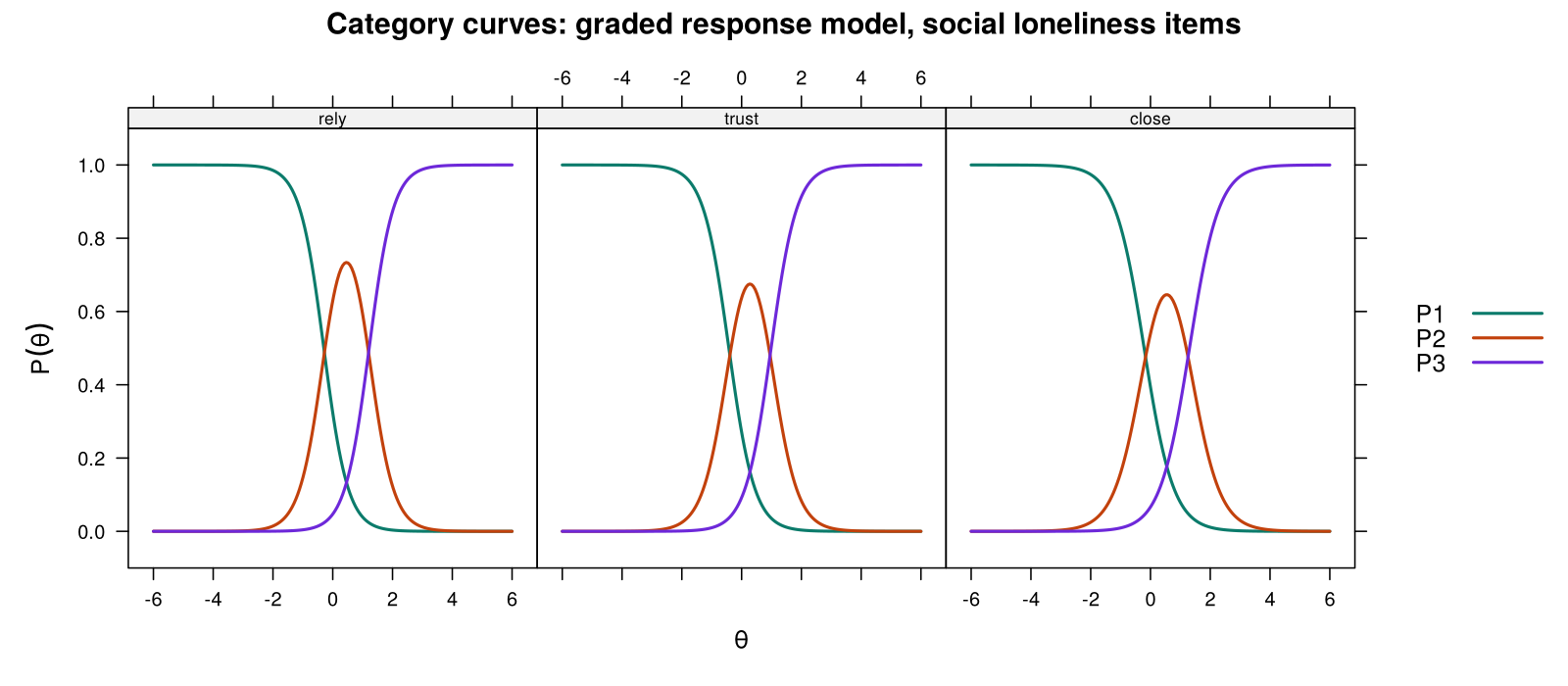
plot(grm, type = "trace")). P1 is the least lonely answer, P2 is "More or less" and P3 is the lonely answer.Item response theory compared with classical test theory
Item response theory and classical test theory describe the same items in different ways and suit different tasks. Table 7.4 compares them on six features, from the unit of analysis to the demands that each places on the analyst.
Table 7.4. Classical test theory and item response theory compared.
| Feature | Classical test theory | Item response theory |
|---|---|---|
| Unit of analysis | The total score | Each item and its curve |
| Precision | One reliability (alpha or omega) for everyone in the sample | Information and standard error that vary along the trait |
| Dependence on the sample | Item statistics and reliability depend on the sample's spread | Item parameters are, in principle, the same in any group in which the model holds |
| Scoring | Sum or mean of item codes | Estimated trait level (θ), which can be compared across different item sets |
| Typical uses | Reporting a scale in a manuscript; short established scales | Building and shortening scales, item banks, computer adaptive tests, testing item bias |
| Demands | Simple to compute and explain | Larger samples, model checks (unidimensionality, local independence) and specialist software |
The graded response model above was fitted to the three social items only, because IRT models of this kind assume that the items measure one trait (unidimensionality), and the factor analysis has shown that the six items measure two. For a manuscript that uses an established scale such as the De Jong Gierveld scale, classical reliability and a confirmatory factor analysis are usually sufficient. Item response theory becomes important when a scale is being built, shortened or compared across groups, and the PROMIS item banks used in health research are a prominent example of its use (Cella et al., 2010).
Worked code 7.1 shows how the graded response model for the three social items was fitted with the mirt package and how Figure 7.9 and Figure 7.10 were drawn.
This box is optional and is not assessed. It shows how the item response curves in the reading were estimated, for anyone who would like to try. It continues from the Section 2 activity and uses the social_items data frame created there. It needs the mirt package, which may take a few minutes to install.
# OPTIONAL: install.packages("mirt")   # run once
library(mirt)
# A graded response model for the three social loneliness items
grm <- mirt(social_items, model = 1, itemtype = "graded", verbose = FALSE)
round(coef(grm, IRTpars = TRUE, simplify = TRUE)$items, 2)Each row is an item. The column a is the discrimination (2.47, 2.32 and 2.03, all steep). The columns b1 and b2 are the thresholds: the trait levels at which the probability of answering above the first and above the second category reaches 0.5. All three items have b1 near −0.2 to −0.4 and b2 near 1.0 to 1.3, so they measure the same part of the trait.
plot(grm, type = "trace")    # category curves for each item
plot(grm, type = "info")     # test information curve
These two lines produce no console output. They draw the category curves and the test information curve shown in Figures 7.10 and 7.9.
Item response theory has described each social item along a continuous trait. The next part introduces latent class analysis, a latent variable model of a different kind.
Latent Class Analysis
Factor analysis and item response theory assume that the latent variable is continuous: people differ by degree along a trait such as loneliness. Latent class analysis is the latent variable model for a categorical latent variable. It assumes that the sample is a mixture of a small number of hidden groups, called latent classes, and that each class has its own probability of each answer to each item (Lazarsfeld & Henry, 1968; Collins & Lanza, 2010). Within a class, the answers to different items are assumed to be unrelated (local independence), so the classes account for all of the association between the items. The model estimates the size of each class and, for every person, a set of class-membership probabilities: the probability of belonging to each class given that person's answers. People are usually placed in their most likely class, and the membership probabilities show how certain each placement is.
The number of classes is chosen by fitting models with one, two, three or more classes and comparing them. The BIC balances fit against the number of parameters, and lower values are preferred, although in large samples it often keeps falling as classes are added. Entropy summarizes how clearly people are assigned to classes, on a scale from 0 to 1, with values near 1 indicating well-separated classes. The size of each class and whether the classes make substantive sense also guide the choice. Factor analysis groups items that measure the same trait, whereas latent class analysis groups people who answer in similar ways.
The card below links to an optional narrated walkthrough that fits latent class models to CSCS data in R.
Optional enrichment: Latent Class Analysis in R
The narrated walkthrough fits models with one to five classes to seven checkbox items from the Canadian Social Connection Survey on what people missed when they felt lonely, compares the models with the BIC, describes the three classes it keeps and assigns each person to a class. It goes beyond the knowledge checks of this lesson.
Open the Latent Class Analysis in R walkthroughThe last part of the section returns from latent variable models to Amira's manuscript and shows how the results of this lesson are reported.
Reporting Measurement in a Manuscript
The Measures paragraph of a manuscript tells readers enough about each scale to judge the scores. It names the scale and its source, describes the items and response options with an example, states the scoring rule (including reverse-coding and any cut-point), reports the reliability observed in the study sample, and summarizes any structural or other validity evidence produced in the study. It also describes how missing items were handled. Claims such as "a validated scale" are replaced by a statement of what was validated, for what use and in which population.
Worked Example 7.2 applies this structure to Amira's manuscript, drawing on the scoring of Section 1, the reliability estimates of Section 2 and the factor analyses of this section. Box 7.14 then describes how the same structure applies to other scales.
Loneliness. Loneliness was measured with the six-item De Jong Gierveld Loneliness Scale (De Jong Gierveld & Van Tilburg, 2006), which contains three emotional loneliness items (for example, "I experience a general sense of emptiness") and three social loneliness items (for example, "There are plenty of people I can rely on when I have problems"), each answered "yes", "more or less" or "no". Following the published scoring rule, each item was scored 1 for "more or less" or the lonely answer and 0 otherwise, taking account of the positive wording of the social items, to give emotional and social subscale scores (0 to 3) and a total score (0 to 6). Participants with any missing item (630 of 4,045) were excluded, leaving 3,415. To test the structure of the scale, the sample was split at random. In the first half (n = 1,708), parallel analysis and an exploratory factor analysis with oblimin rotation supported two factors. In the second half (n = 1,707), a two-factor confirmatory model fitted acceptably (CFI = 0.949, TLI = 0.905, RMSEA = 0.082, SRMR = 0.060) and considerably better than a one-factor model (CFI = 0.739, RMSEA = 0.177; chi-square difference = 386.95, df = 1, p < 0.001). Internal consistency, computed from the three-point item codes, was adequate for the social subscale (Cronbach's alpha = 0.75; McDonald's omega = 0.75) and low for the emotional subscale (alpha = 0.51; omega = 0.57), in which the item "I miss having people around me" loaded weakly (standardized loading 0.20). We therefore report the two subscales separately as well as the total, interpret associations with emotional loneliness as likely underestimates, and present a sensitivity analysis using the two remaining emotional items.
Box 7.14: Applying the worked example to other scales
The same structure serves any multi-item scale. A Measures paragraph names the scale and cites its development paper, gives one example item and the response options, states the scoring rule and any reverse-coding, reports alpha and omega computed in the study sample, and describes how missing items were handled. When the research question depends on the subscales of a scale, or a reviewer could reasonably question its structure, it adds a confirmatory factor analysis with the four fit indices. The Factor Analysis and Scale Scoring walkthrough and the answer key for this lesson contain the code for each step.
Worked Example 7.2 completes Amira's reply to the reviewer. It reports that the six items measure two related constructs and that the social subscale has adequate internal consistency and the emotional subscale low internal consistency, and it states how the analysis takes account of both findings. The knowledge check and reflection that follow review the material of this section, and the Key Takeaways and final assessment of the lesson bring the four sections together.
1. In a standardized factor model, an item has a loading of 0.70 on its factor. What share of the item's variance does the factor explain?
2. Parallel analysis is used in exploratory factor analysis to:
3. A confirmatory model has CFI = 0.97, TLI = 0.96, RMSEA = 0.04 and SRMR = 0.03 in a sample of 2,000, and its chi-square test has p < 0.001. Which conclusion is best?
4. In item response theory, the difficulty parameter b of a 0 or 1 item is:
5. Which statement best compares item response theory with classical test theory?
✎ Reflection
A confirmatory factor analysis tests whether items load on the factors that theory assigns them to. Model fit is judged with four indices, using common guides for good fit: the comparative fit index (CFI, 0.95 or higher), the Tucker-Lewis index (TLI, 0.95 or higher), the root mean square error of approximation (RMSEA, 0.06 or lower, with up to 0.08 often called acceptable) and the standardized root mean square residual (SRMR, 0.08 or lower). In half of the 2021 Canadian Social Connection Survey sample (1,707 people), a two-factor model of the six De Jong Gierveld items (an emotional factor with three negatively worded items and a social factor with three positively worded items) gave CFI = 0.949, TLI = 0.905, RMSEA = 0.082 and SRMR = 0.060. A one-factor model gave CFI = 0.739, TLI = 0.565, RMSEA = 0.177 and SRMR = 0.110, and the chi-square difference test favoured two factors (p < 0.001). The standardized loadings were 0.82, 0.20 and 0.57 on the emotional factor (the 0.20 item is "I miss having people around me") and 0.75, 0.73 and 0.65 on the social factor, and the factors correlated 0.25. A reviewer asked whether the six items measure one construct or two. Write the paragraph you would send in reply (five to seven sentences), stating your conclusion, the evidence for it, two limitations, and what you will change in the analysis.
Lesson 7: Final Assessment
Bringing It All Together
This lesson took the analyst's view of the multi-item scales that most analyses of the CSCS use. Section 1 traced the chain from a construct, through its domains and items, to an instrument and a scoring rule. It separated reflective scales, whose items are caused by the construct and are expected to correlate, from formative indices, whose components define the construct. It prepared and scored the six De Jong Gierveld items in R, including the reversal of the three positively worded items, and introduced classical test theory, in which reliability is the true-score share of observed variance and measurement error weakens correlations.
Section 2 estimated reliability. A single survey supports only internal consistency, and in the CSCS the social subscale had an alpha and an omega of 0.75 while the emotional subscale had an alpha of 0.51 and an omega of 0.57, with one weak item. Alpha rises with the number of items, assumes equal loadings, cannot show that a scale is unidimensional and has no meaning for an index, and it fell from 0.59 to 0.42 when the reversal step was skipped. Section 3 treated validity as an argument for a stated use in a stated population, organized the evidence with the COSMIN taxonomy, and found convergent, discriminant and known-groups evidence that supports the scale and distinguishes its two subscales. Section 4 used exploratory factor analysis in one half of the sample and confirmatory factor analysis in the other to show that two related factors (CFI 0.949, RMSEA 0.082) fit far better than one (CFI 0.739, RMSEA 0.177), and it introduced item response theory, in which each item has a curve and precision varies along the trait.
Together these steps answered both of the reviewer's questions and produced a Measures paragraph that reports the scale's source, scoring, reliability in the study sample and structural evidence. The final assessment asks for these steps to be applied to new scales. The next lesson, Mediation, Moderation and Path Analysis, extends the confirmatory factor model of Section 4 into path models and structural equation models.
Key Takeaways from this lesson
- A score is linked to its construct through domains, items, an instrument and a scoring rule, and a Measures paragraph describes each link.
- The items of a reflective scale are expected to correlate, whereas the components of a formative index need not, so internal consistency applies only to scales.
- Reverse-worded items must be recoded according to the scoring manual before items are combined.
- Classical test theory defines reliability as the true-score share of observed variance, and unreliable measures weaken observed associations.
- Cronbach's alpha rises with the number of items, assumes equal loadings and cannot show unidimensionality, so McDonald's omega is reported alongside it.
- Validity is an argument for a stated use in a stated population, built from content, criterion, construct and structural evidence.
- Exploratory factor analysis suggests a structure, and confirmatory factor analysis tests it in data the exploration did not use, judged with the CFI, TLI, RMSEA and SRMR.
- Item response theory describes each item with a curve defined by its difficulty and discrimination, and gives precision that varies along the trait.
The final assessment covers all four sections. All 15 questions must be answered correctly (100%), and the final reflection completed, to finish the lesson.
Reflection
A student plans to use a hypothetical eight-item Neighbourhood Belonging Scale in a manuscript based on an online survey of 2,400 adults. Each item is answered on a five-point scale coded 1 (strongly disagree) to 5 (strongly agree). Five items are worded so that agreement means more belonging, and three items (for example, "I feel like an outsider on my street") are worded so that agreement means less belonging. The published scoring rule sums the eight items after reverse-coding, giving a total from 8 to 40. In the student's sample, after correct reverse-coding: alpha for all eight items is 0.78; parallel analysis suggests two factors; in a random half of the sample, a one-factor confirmatory model gives CFI = 0.86, TLI = 0.80, RMSEA = 0.11 and SRMR = 0.07, and a two-factor model (a five-item "attachment" factor and a three-item "exclusion" factor made of the negatively worded items) gives CFI = 0.97, TLI = 0.96, RMSEA = 0.05 and SRMR = 0.03, with a factor correlation of 0.62. Alpha is 0.84 for the attachment items and 0.68 for the exclusion items. The total score correlates 0.45 with a measure of neighbourhood social cohesion and 0.12 with household income, and people who have lived in their neighbourhood for more than five years score higher than newer residents. Common guides for good fit are CFI and TLI of 0.95 or higher, RMSEA of 0.06 or lower and SRMR of 0.08 or lower. Write the Measures paragraph for this scale (six to eight sentences). Include the reverse-coding formula, the reliability results, the structural evidence and the validity evidence, state one limitation that the structure of the scale raises, and do not describe the scale as simply "validated".
Minimum 20 characters required.
Final Knowledge Assessment
1. Which of the following is best described as a formative index?
2. A researcher sums ten items without reversing the four positively worded ones. Which consequence is most likely?
3. The true correlation between two constructs is 0.40. They are measured with reliabilities of 0.81 and 0.64. What observed correlation is expected?
4. A study administers a scale once, online, to 3,000 people. Which kind of reliability can it estimate from its own data?
5. A 15-item scale has alpha = 0.97. What is the most reasonable concern?
6. In psych::alpha() output, the r.drop value for an item is:
r.drop is the corrected item-total correlation, the correlation between the item and the total of the remaining items. Alpha after removal appears in the separate Reliability if an item is dropped table.7. For a three-item subscale with standardized loadings of 0.85, 0.25 and 0.60, how will alpha compare with omega?
8. A colleague writes that "the scale is valid". Which revision best reflects the argument-based view of validity?
9. Scores on a new physical activity scale are higher among marathon runners than among office workers who report no exercise. This is an example of:
10. A loneliness scale correlates 0.62 with another loneliness scale and 0.20 with extraversion. How is this pattern best described?
11. Before an exploratory factor analysis, the KMO measure is 0.82. What does this suggest?
12. Why is an oblique rotation such as oblimin usually preferred for health constructs?
13. A confirmatory model gives CFI = 0.91, TLI = 0.88, RMSEA = 0.10 and SRMR = 0.09. Using common guides, how should its fit be described?
14. In lavaan syntax, what does the line support =~ q1 + q2 + q3 specify?
=~ is read as "is measured by", so the line defines a latent factor called support with q1, q2 and q3 as its indicators.15. A test information curve is high between θ = 1 and θ = 3 and close to zero below θ = 0. What does this imply?
✦ Before submitting: pass every section knowledge check (100%) and complete every reflection.