Computational Text Analysis, Cultural Domain Analysis & LLM-Assisted Coding
The Final Lesson
Learning objectives for this lesson:
- Apply keyword-in-context (KWIC), word-frequency, keyness, and collocation analysis to interview corpora
- Distinguish TF-IDF, keyness (chi-squared/log-likelihood), and raw frequency, and select the right measure for the analytic question
- Conduct cultural domain analysis, free listing (with Smith's salience), pile sorts (with MDS), triad tests, and the Romney-Weller-Batchelder consensus model
- Build a term co-occurrence network, compute centrality and community structure, and visualize it
- Articulate the opportunities and risks of LLM-assisted qualitative coding, speed, scale, reproducibility, hallucination, prompt drift, bias amplification
- Design a calibration-and-validation workflow for LLM coding using a hand-coded reference set and Krippendorff's alpha
- Write a prompt that applies a study codebook reliably to a transcript, and audit the resulting codings
- Disclose the use of LLM tools defensibly in a methods section
- Check that consent, terms of use, and privacy law permit a model to process interview transcripts before any are uploaded
This course was developed by Dr. Kiffer G. Card, Faculty of Health Sciences, Simon Fraser University based on Bernard, H. R., Wutich, A., & Ryan, G. W. (2017). Analyzing Qualitative Data: Systematic Approaches (2nd ed.). SAGE. This lesson covers Chapters 17, 18, and 19, and extends to LLM-assisted coding, a methodology that postdates Bernard, Wutich, and Ryan’s 2017 edition and is the most rapidly changing topic in the field.
KWIC, Word Counts, and Keyness Analysis
Introduction and Overview
For the first eleven lessons of this course you have read transcripts line by line, hand-coded passages in Taguette, built codebooks, compared subgroups, written analytic memos, and worked your way through grounded theory, content analysis, schema analysis, narrative analysis, discourse analysis, and analytic induction. All of that work is what Bernard, Wutich, and Ryan call close reading. It is irreplaceable. But it does not scale. A 20-transcript loneliness corpus is at the upper edge of what a single analyst can read three or four times during a single graduate term. A 200-transcript corpus is not analyzable in that way. A 20,000-document corpus, the kind that increasingly arrives from social-media scraping, electronic health-record narrative fields, or large-scale open-text survey items, is unanalyzable in that way for any human team.
Computational text analysis is the family of techniques that lets you ask quantitative questions of a text corpus without first reducing the texts to codes (Grimmer, Roberts, & Stewart, 2022; Wikipedia contributors, n.d.-a). The questions are simple: which words appear most often? which words appear distinctively in subgroup A compared to subgroup B? which words travel together? where in the corpus does a given word appear, and in what immediate context? The answers are computed in seconds for corpora the size of yours and in minutes for corpora a thousand times the size. Chapter 17 of Bernard, Wutich, and Ryan covers the foundational techniques: keyword-in-context (KWIC), word frequencies, type-token ratios, TF-IDF, keyness, collocations, and n-grams. This first section of this lesson walks you through each of them, applied to the loneliness corpus.
One framing point before we begin. Computational text analysis is sometimes presented as an alternative to close reading. It is not. Bernard, Wutich, and Ryan's stance, and the stance of this course, is that computational techniques are front-loaders for close reading. They surface candidates for the analyst to read, in context, and decide whether the pattern is real. A keyness analysis that identifies tired as significantly more frequent in older participants than in younger participants is not a finding. It is a pointer toward passages worth reading closely. The finding is what you say after you have read those passages and decided whether the word is doing analytically interesting work or simply registering a generational vocabulary tic.
Learning Objectives for this section
- Apply keyword-in-context (KWIC) analysis to the loneliness corpus.
- Compute and interpret word frequencies, type-token ratios, and lexical diversity.
- Distinguish raw frequency, TF-IDF, and keyness, and select the right measure for an analytic question.
- Interpret a keyness analysis comparing older and younger participants in the loneliness corpus.
- Identify collocations (words that co-occur more often than chance).
- Understand n-grams as multi-word features and when to use them.
1.1 KWIC: The Oldest Computational Text-Analysis Technique
Keyword in Context. The oldest computational text-analysis technique, dating to medieval concordances and computerized in the 1950s. Generates lists of every occurrence of a target word with surrounding context. Used to disambiguate polysemy and to see how a term is actually deployed in a corpus before interpreting frequency counts.
Term Frequency × Inverse Document Frequency. A weighting that boosts terms frequent in a particular document and penalizes terms common across the whole corpus. Surfaces what is distinctive about each document. The standard input to document classification and retrieval systems.
Keyness. Statistical comparison of word frequencies in a target corpus vs a reference corpus. 'Which words are unusually frequent in 2026 health policy documents compared to 2010?' Log-likelihood and chi-squared tests are common. Output: a ranked list of distinguishing terms.
Collocations: words that co-occur within a defined window more often than chance would predict ('mental + health', 'public + health'). N-grams: consecutive word sequences (2-grams, 3-grams). Both reveal multi-word concepts that single-word analysis misses.
The keyword-in-context concordance is the oldest digital text-analysis technique, predating personal computers. The original KWIC concordances were produced on mainframes in the 1950s and 1960s, most famously for biblical scholarship and for early lexicography (Bernard, Wutich & Ryan, 2017, Ch. 17). The idea is simple: pick a target word; for every occurrence of that word in the corpus, print the word plus a fixed number of words on either side. The output is a vertical list of one-line excerpts with the target word column-aligned in the middle. A human can scan a 200-line KWIC of a single word in two or three minutes and develop a sense of how the word is being used that no other technique offers as cheaply.
The reason KWIC remains analytically valuable in 2026 is that it does something that quantitative text statistics do not: it preserves local context. A word frequency table tells you that chair appears 47 times in the loneliness corpus; it does not tell you that 32 of those 47 are references to a chair where an absent person used to sit, that 11 are references to the participant's own seated immobility, and that 4 are incidental mentions of furniture. The KWIC reveals the distribution of senses in seconds. The numerical-frequency analyst who skipped the KWIC step might mistakenly write “chairs are an important physical motif in the loneliness corpus,” which is true but misses the more specific finding that empty chairs are an important physical motif.
The technical mechanics of KWIC are trivial. The interpretive demands are not. A good KWIC reading is one where you have looked at every line of the concordance, classified each occurrence into a small number of senses, and decided which sense is the analytically productive one. You should treat KWIC as a five-to-ten-minute exercise per target word, not as a one-line command whose output you skim.
To try KWIC on the loneliness corpus, open the 20 transcripts in the course data bundle, HSCI_841_loneliness_data.zip, search each one for chair, and copy every occurrence with about six words on either side into a single list. Read the list line by line and classify each occurrence into a sense (the empty chair of an absent person, the participant’s own chair as a marker of immobility, an incidental mention of furniture); the distribution of senses is itself a finding. Repeat the exercise for alone and lonely. Bernard, Wutich, and Ryan (and your transcripts) treat these as distinct, and a KWIC contrast surfaces the distinction concretely.
1.2 Word Frequencies, Type-Token Ratios, and Lexical Diversity
The simplest computational text statistic is the word frequency. After removing stopwords (the, and, of, but, was, are…), you compute how many times each remaining word appears in the corpus and rank them. The top 50 or 100 words are usually a mix of the obvious (loneliness, alone, people, feel) and the surprising. The surprising ones are the analytically valuable findings. In the loneliness corpus, the top 50 content words include chair, quiet, radio, wednesday, and fading; each of those repays a KWIC read and yields a candidate theme.
Word frequency analysis is also the foundation for two further statistics: the type-token ratio (TTR) and lexical diversity. A token is any occurrence of a word; a type is a distinct word. The phrase “the chair, the empty chair” contains 5 tokens and 3 types (the, chair, empty). The ratio of types to tokens is one measure of how lexically varied a text is. A high TTR means the speaker uses many different words; a low TTR means they recycle a small vocabulary. TTR is sensitive to document length (longer documents inevitably have lower TTRs because common words repeat), so for cross-document comparison you typically use a length-corrected measure such as the Moving-Average Type-Token Ratio (MATTR) or Mean Segmental TTR (MSTTR).
In health research, lexical diversity has been used as a coarse proxy for cognitive function (lower diversity in dementia transcripts) and for emotional constriction (lower diversity in some depression measures). In your loneliness corpus, a comparison of lexical diversity across participants is a defensible analytic move, it would let you ask, for example, whether the participants with the most circumscribed social worlds also speak with the most circumscribed vocabularies. Bernard, Wutich, and Ryan would emphasize that any such finding requires close-reading confirmation; a numerical difference is a pointer, not a conclusion.
What to look for: the top-50 list of content words surfaces the candidate words for KWIC analysis. A ranking of participants by MATTR identifies the participants with the most and least varied vocabularies. Read those transcripts again in light of their MATTR rank, and decide whether the numerical difference registers something analytically meaningful (a genuine constriction of social or emotional vocabulary) or a stylistic or dialectal difference.
1.3 TF-IDF: Term Frequency × Inverse Document Frequency
Raw word frequency tells you which words appear most often in the corpus. It does not tell you which words are distinctive of a particular document. The word loneliness appears many times in every transcript; it is not informative about which transcript is which. The word wahda appears in only one transcript (P15, Amira) and there several times; it is highly informative about that transcript.
Term Frequency × Inverse Document Frequency (TF-IDF) is the classical measure designed to surface this kind of document-distinctive vocabulary (Wikipedia contributors, n.d.-b). The idea is to weight each word's frequency in a document by how rarely it appears in the rest of the corpus. The term-frequency component rewards words that are common in the focal document; the inverse-document-frequency component penalizes words that are common in many other documents. The product is highest for words that are common in this document and rare elsewhere. TF-IDF was developed for information retrieval (which documents are most relevant to a search query?) in the 1970s and has become the workhorse statistic for document similarity, search ranking, and feature selection in supervised text classification.
In qualitative analysis, TF-IDF is most useful for surfacing what a single transcript is distinctively about. A TF-IDF ranking of P15 (Amira, recent refugee from Syria) is likely to surface wahda, Aleppo, family, before, and other terms that capture what is distinctive about Amira's account of loneliness compared to the other nineteen participants. Bernard, Wutich, and Ryan treat this as a tool for case characterization: which words best describe what makes this case different from the rest of the corpus?
Ranking each transcript’s words by TF-IDF gives a vocabulary fingerprint for each participant. In the loneliness corpus, P15 (Amira) surfaces wahda and Syria-related terms; P11 (Helen) surfaces fading, radio, marie, and wednesday; and P05 (Linda) surfaces terms tied to her widowhood and her terrier. These fingerprints are useful both as descriptive case sketches in your findings section and as cross-checks on the candidate themes that emerged in earlier coding.
1.4 Keyness: Comparing Two Subcorpora
Keyness analysis is the comparative cousin of TF-IDF. Instead of asking which words distinguish a single document from the corpus, it asks which words distinguish a group of documents (a subcorpus) from another group of documents. The standard implementation uses either the chi-squared test or the log-likelihood ratio test on the 2×2 frequency table of (word X / not-word X) by (group A / group B), one word at a time. The output is a ranked list of words with their test statistic, p-value, and frequency in each subcorpus. The words at the top are the words that are statistically more distinctive of one subcorpus than the other.
Keyness is widely used in corpus linguistics (e.g., comparing British versus American English corpora) and increasingly in health research (comparing patient-experience text by diagnosis, by gender, by treatment arm in a trial). For your loneliness corpus, the most natural comparison is across age. The corpus contains four participants in their seventies and eighties (P05 Linda, P11 Helen, P17 Jacob, P20 Frank) and four in their twenties (P01 Maya, P10 Daniel, P12 Tyler, P19 Rose). A keyness analysis comparing these two subcorpora surfaces the vocabulary of late-life loneliness against the vocabulary of early-adult loneliness, and the contrast is consequential. The older subcorpus has more keywords like dead, quiet, visit, fading, radio, walker; the younger has more keywords like online, screen, followers, group chat, discord, scrolling.
The interpretive point is not that the words are themselves the finding. The interpretive point is that the structural worlds in which the two cohorts experience loneliness are different, and the keyness list is a vocabulary-level signature of that structural difference. The finding the keyness analysis points you toward, that the technology mediation of loneliness in young adulthood and the embodied immobility of loneliness in old age are different empirical objects deserving different policy responses, is the analytic claim that goes in the write-up. The keyness list is the evidence trail.
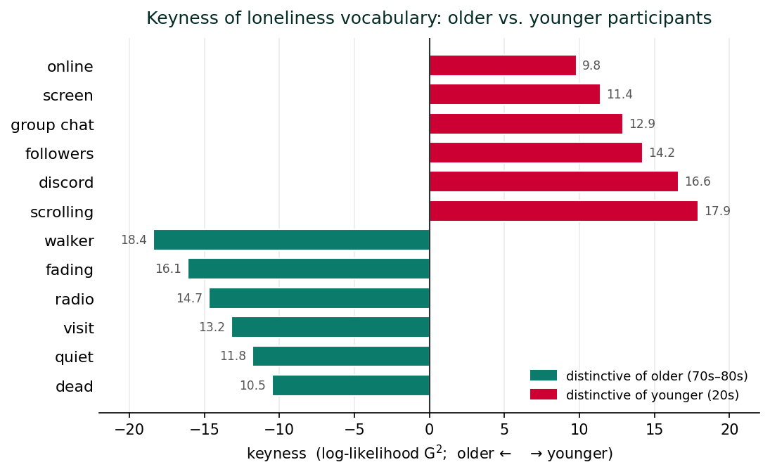
Two interpretive cautions apply to the figure above. First, keyness with small subcorpora (four documents per group) is statistically fragile, so individual word p-values are best treated as pointers to passages, with confirmation left to the close read. Second, read every keyword in its KWIC context before drawing any interpretive conclusion. The numerical contrast is the front end; the close read is the analysis.
1.5 Collocations: Words That Travel Together
A collocation is a pair (or larger sequence) of words that co-occurs more often than chance would predict. The standard test is again log-likelihood or chi-squared on the 2×2 contingency table of (word A present / absent) by (word B present / absent) within a sliding window of n words. High-scoring collocations tell you which word pairs are linguistically bonded in the corpus. The output for a loneliness corpus might include empty chair, quiet apartment, group chat, tired all the time, nobody there, last conversation, and similar pairings.
Collocations are useful for two analytic purposes. First, they surface candidate multi-word concepts that single-word frequency analysis misses. Empty chair as a collocation captures something neither empty nor chair alone does; it is the unit of meaning. Second, they surface candidate conventional metaphors, recurring word combinations that participants are drawing on a shared symbolic vocabulary to use. In the loneliness corpus, recurring phrases like fading at the edges (Helen), shrinks around you (also Helen), and empty space (multiple participants) are conventional metaphors in the Lakoff-Johnson sense; collocation analysis surfaces them efficiently.
Comparing the words that fall within a few words of alone with those that fall near lonely makes the contrast visible. The alone neighborhood tends to surface neutral or even positive context words (home, quiet, peace, comfortable), because participants describe being alone in many ways and only some of them are lonely. The lonely neighborhood tends to surface affectively heavier neighbors (tired, hollow, fading, empty, dead, miss). The contrast operationalizes Bernard, Wutich, and Ryan’s claim, and your participants’ direct statements, that alone and lonely are distinct concepts.
1.6 N-grams
An n-gram is a sequence of n consecutive words. Unigrams (n=1) are single words; bigrams (n=2) are pairs; trigrams (n=3) are triples. The collocations above were a special case of n-grams: bigrams and trigrams whose components co-occur statistically more than chance. Plain n-gram frequency analysis, without the statistical-collocation filter, is also useful, especially when you want to find conventional fixed phrases (at the end of the day, most of the time, I don't know) or when you are setting up a more elaborate downstream model that consumes n-gram features (a topic model, a supervised classifier, a semantic network on bigrams).
Technically, an n-gram feature set is built by joining each run of n consecutive words into a single feature (for example, empty_chair) and then counting those features like any other words. The cost is that the resulting feature space is much larger than the unigram space (typically 10–20× more features), which slows downstream computation; the benefit is that n-grams capture lexical structure that unigrams cannot.
1.7 What These Techniques Do and Do Not Tell You
Computational text statistics are useful diagnostics. They are not, on their own, qualitative analysis. Bernard, Wutich, and Ryan are explicit on this: a frequency table, a keyness list, a TF-IDF ranking, and a collocation report are pointers. They surface candidates for close reading. The analytic move, deciding what the patterns mean, whether they support a theme, whether they tell you something about the phenomenon or merely about the vocabulary your participants happen to share, remains the analyst's work. Treat this section's tools as the first hour of a longer day. They tell you where to look. The looking is still your job.
Reflection
Of the techniques in this section, KWIC, frequency, TTR/MATTR, TF-IDF, keyness, collocations, which one would be most analytically useful for a specific research question about the loneliness interviews? Why? Be specific about what it would surface and how that would feed into a close-reading move.
Minimum 20 characters required.
Question 1: Which of the following is the analytically most defensible use of a keyness analysis comparing older and younger participants in the loneliness corpus?
Question 2: Why is raw word frequency a poor measure for surfacing the words most distinctive of a single transcript?
Question 3: KWIC analysis is most accurately described as:
Cultural Domain Analysis: Free Lists, Pile Sorts, Triads, Consensus
Introduction and Overview
Cultural domain analysis is a family of techniques developed in cognitive anthropology in the 1950s through 1980s to study how people in a cultural group mentally organize a delimited domain of knowledge: kinds of illness, kinds of edible plants, kinds of kin, kinds of risk. The starting premise is that a cultural domain is a shared mental model. The techniques in this section, free listing, pile sorts, triad tests, and consensus analysis, are designed to measure the structure of that shared model and to estimate each participant's degree of competence: how closely their understanding of the domain tracks the group consensus.
For public-health audiences, cultural domain analysis is consequential because most health categories (kinds of risk, kinds of symptom, kinds of treatment, kinds of support) are domain-organized in exactly this way. A public-health communication campaign that treats “the public” as a single audience with a single mental model often fails because the model is in fact heterogeneous across groups. Cultural domain analysis measures the heterogeneity precisely and tells you which sub-populations share a model and which do not.
The intellectual lineage is short and important. The technique was systematized by Romney, Weller, and Batchelder in their 1986 paper Culture as Consensus: A Theory of Culture and Informant Accuracy, published in American Anthropologist. The Romney-Weller-Batchelder (RWB) consensus model treats culture statistically: there is a true cultural answer for each item in the domain, and participants approximate it with varying competence. The model estimates competence from inter-informant agreement (using a factor-analytic decomposition) and produces, for each item, a best-estimate cultural answer that is the competence-weighted average of all participants' answers. The model has been applied to hundreds of public-health questions, from kinds of risk for HIV transmission to the cultural domain of acceptable cooking fuels in low-income households.
Learning Objectives for this section
- Conduct a free-listing exercise and compute Smith's salience.
- Distinguish single-sort and successive-sort pile sorts, and analyze pile-sort data with multidimensional scaling (MDS).
- Conduct a triad test and read its output.
- State the Romney-Weller-Batchelder consensus model assumptions and interpret the eigenvalue ratio test for cultural agreement.
- Apply cultural domain methods to a public-health question: which dimensions of social support, kinds of risk, or kinds of treatment do your participants share a model of?
2.1 Free Listing: The Foundational Elicitation Technique
Ask 30+ informants to list all the items they can think of in a domain. Aggregate the lists. Two key outputs: (1) salience scores per item (frequency + rank), (2) the empirical map of the domain’s vocabulary. Most cultural-domain studies start here.
Give informants 20-40 items (typically from free lists) and ask them to sort into piles. Aggregate proximity matrices. Multidimensional scaling and hierarchical clustering reveal the implicit category structure. The result is a map of how the domain hangs together.
Present three items and ask which one doesn’t belong. Repeated across many triads, this elicits the underlying dimensions along which informants distinguish items. More cognitively demanding but more discriminating than pile sorts; useful for refining a known structure.
A statistical model that uses the pattern of agreement across informants to (a) estimate each informant’s competence in the domain, (b) estimate the ‘answer key’ that the group implicitly shares. The defensible alternative to majority voting in cultural surveys. Particularly important when cultural consensus itself is the research question.
Free listing is the simplest cultural domain technique and almost always the one to start with. You ask a participant a simple prompt: “List all the kinds of X you can think of.” You let them list freely, in their own order, for as long as they wish to continue. You record both the items and the order. You collect free lists from a sample of n participants (typically 20–40 is sufficient; less than 15 is usually too few for reliable salience estimates). You then analyze the combined list to identify (a) which items are mentioned by the most participants (frequency), (b) which items tend to be mentioned early (rank), and (c) which items are both common and early (Smith's salience).
Smith's salience is a single number per item, calculated as:
S = ( ∑ ((L − Rp + 1) / L) ) / N
where, for each item, you sum across the N participants the quantity (L − Rp + 1) / L, with L being the length of participant p's list and Rp being the rank of the item in that list (R = 1 for first-mentioned). The numerator gives full credit (= 1) to an item mentioned first on a participant's list, half credit to an item halfway down the list, and so on. The sum is divided by N (the total number of participants). The resulting score ranges from 0 to 1; higher is more salient.
Items with the highest Smith's salience are the core items of the domain, the ones a randomly chosen member of the group is most likely to think of first when asked about the domain. Items with low salience are peripheral, idiosyncratic to one or two participants, or sub-domain-specific. In a free-listing exercise on “kinds of social support,” the high-salience items might be family, friends, partner; the low-salience items might be online community, religious community, therapist. The contrast tells you what the participants' default model of social support contains, and what they leave out.
The loneliness interviews are semi-structured rather than free-list, but several questions in the interview guide elicit list-like responses (Domain 2, Q7: “Are there situations or times that reliably bring it on?”; Domain 4, Q11: “What helps?”). For the worked example below, treat each participant's response to Q11 (“What helps?”) as their free list of coping strategies. Extract the items mentioned and their order. Compute Smith's salience across the 20 participants. The high-salience items are the cultural core of coping with loneliness in this sample; the low-salience items are idiosyncratic.
A real free-listing study would use the prompt “List all the things that help you when you are lonely” and would record the listing directly. The retrospective extraction from semi-structured interviews is a defensible second-best.
Smith’s S can be computed by hand or in a spreadsheet. For each participant’s list, give each item the score (L − R + 1) / L, add each item’s scores across participants, and divide by the number of participants, so that participants who did not list an item contribute 0.
The course data bundle, HSCI_841_loneliness_data.zip, includes the free lists extracted from the 20 transcripts (freelist_what_helps.csv), with one row per participant, item, and rank. The 20 lists name 31 different items, with an average list length of 4.25. The five most salient items are shown below.
| Item | Participants listing it (n / 20) | Smith’s S |
|---|---|---|
| peer-group | 10 | 0.43 |
| therapy | 9 | 0.25 |
| friends | 6 | 0.22 |
| television | 5 | 0.14 |
| cooking | 3 | 0.11 |
Peer groups stand out as the cultural core of coping in this sample: half the participants name one, usually near the top of their list. Therapy is listed almost as often but further down the lists, which lowers its salience. Most of the remaining items are named by one to four participants and sit in the periphery. For a public-health intervention designer, the cultural core tells you what most people will already know about; the periphery tells you what an information campaign would need to introduce.
2.2 Pile Sorts: Eliciting Implicit Structure
A pile sort is conducted as follows. You write each item of the domain on a card (or display them on a screen). You hand the deck to a participant and say: “Sort these into piles so that the things in each pile are similar to each other. Make as many or as few piles as you like.” You record the resulting partition: which items the participant placed together. You repeat across n participants and aggregate the pile sorts into a single similarity matrix: cell (i, j) of the matrix is the number of participants who put items i and j in the same pile.
The aggregate similarity matrix is then analyzed with multidimensional scaling (MDS) or hierarchical clustering to recover the implicit structure of the domain. MDS produces a 2-D map where items are points and the distances between them reflect their dissimilarity. Items that participants reliably grouped together appear close on the map; items that were almost never grouped together appear far apart. The resulting map is the visualization of the group's shared mental structure of the domain.
A successive pile sort is the same exercise repeated: after the first sort, you ask the participant to combine piles (“Which of these piles could be combined into a larger pile? Which combinations would still feel similar?”) until they reach a small number of super-piles, and you record the hierarchy. The result is a hierarchical clustering for each participant, which can also be aggregated. The successive pile sort is more informative than the single sort but slower; the single sort is the standard for most studies.
For a worked example consistent with the loneliness study: imagine 30 cards, each naming a kind of social relationship (mother, father, sibling, partner, best friend, ex-partner, coworker, neighbour, pet, online friend, religious-community member, therapist, GP, phone-pal, group-chat acquaintance, …). A pile-sort study with 25 BC residents would produce an MDS map of how these relationships cluster in our shared mental model. The clustering would tell you which relationships participants treat as functionally equivalent for the purpose of countering loneliness, which they treat as substitutes, and which they treat as categorically different. Such a study would be policy-actionable: if “pet” clusters with “close friend” in the shared model, then a pet-based intervention is closer to the cultural category of friendship than to the cultural category of distraction, with consequences for how the intervention is framed and evaluated.
The course data bundle includes a small pile-sort dataset (pilesort_relationships.csv) in which 20 participants sorted ten kinds of social relationship into piles. Counting, for every pair of items, how many participants placed the two in the same pile gives the similarity matrix, and classical MDS of that matrix (available in most statistical packages) gives a two-dimensional map. In this dataset the three kin items (mother, partner, adult child) sit together, the three close non-kin items (best friend, neighbour, support group) form a second cluster, the three mediated ties (coworker, group chat, online friend) form a third, and pet sits on its own, which is the interesting result.
The algorithm does not label the dimensions of the map. Part of your analytic work is to inspect the map and propose a labelling (for example, dimension 1 = “intimacy”, dimension 2 = “embodiment”). Proposed dimensional labels are an interpretive claim that needs argument, and they come from the analyst.
2.3 Triad Tests
The triad test addresses a methodological problem with pile sorts: pile sorts assume participants can hold and partition an entire deck of items at once, which is cognitively heavy for large decks. The triad test breaks the problem into manageable pieces. You present three items at a time and ask: “Which of these three is most different from the other two?” (Some variants instead ask which two are most similar; the information is equivalent.) Across many triads, you accumulate enough pairwise-similarity data to reconstruct the same kind of similarity matrix that the pile sort produces, but with finer resolution.
The cost is the number of triads. For a domain of n items, there are C(n, 3) = n!/(3!(n−3)!) possible triads; for n = 15, that is 455 triads, which is too many for any participant to complete. Triad-test designers use balanced incomplete block designs (Borgatti's UCINET implementation has a wizard for this) that present each participant with a stratified subset of triads such that every pair of items appears in approximately equal numbers of triads across the sample. The standard analysis is again MDS on the aggregated similarity matrix.
Triad tests have largely been displaced in contemporary practice by pile sorts (which are faster) and by ratings (which are easier to administer remotely). They remain the gold standard for very small domains (n < 10) and for studies where the cognitive load of holding the full deck would compromise data quality (children, participants with cognitive impairment).
2.4 Consensus Analysis: The Romney-Weller-Batchelder Model
The pile sort and the triad test produce an aggregate similarity matrix for the group. The Romney-Weller-Batchelder consensus analysis goes one step further: it treats the participants themselves as items to be analyzed, and asks how much do they agree with each other? The output is two-fold: a per-participant competence score (how closely the participant's answers track the group consensus) and an estimated cultural answer for each item (the competence-weighted average of all participants' answers).
The model has three formal assumptions: (1) there is a single shared cultural truth for each item in the domain (one knowledge system, not several); (2) participants' answers are independent samples from their own competence-driven approximation to the truth; (3) each participant's competence is approximately constant across items. The first assumption is the most consequential and the most testable. If the data violate assumption 1, if there are two or more distinct cultural sub-models in your sample, the consensus analysis will tell you so.
The diagnostic is the eigenvalue ratio test. Consensus analysis runs a factor analysis on the participant-by-participant agreement matrix. If there is a single shared culture, the first eigenvalue will be much larger than the second, the rule of thumb is that the first should be at least three times the second. If the first/second ratio is closer to 1, there is no single consensus; the sample contains multiple sub-cultures. In that case you should not report a single “cultural answer”; you should report separate analyses for each subgroup (and explain in your discussion why the consensus broke down).
In contemporary public health, consensus analysis has been used to study, among other things, lay theories of HIV transmission risk in different communities (where the eigenvalue ratio test repeatedly identifies sub-cultures), kinds of postpartum mood, kinds of acceptable harm-reduction supply, and the cultural domain of “a good death.” The technique's strength is that it gives a formal statistical test for whether your participants share a cultural model; its weakness is the strong single-culture assumption and the modest sensitivity of the eigenvalue test in small samples.
The course data bundle includes a consensus dataset (consensus_loneliness.csv) in which the 20 participants answer 12 yes/no statements about loneliness. The computation follows the model directly. The agreement matrix records, for each pair of participants, the proportion of statements on which they give the same answer. Its eigen-decomposition gives the eigenvalue ratio and each participant’s competence (the participant’s loading on the first factor), and the cultural answer for each statement is a competence-weighted vote. If the ratio of the first to the second eigenvalue is at least 3, the sample supports a single-culture model and the cultural answers can be read as the group’s best estimate of the truth for each item. If the ratio is between 2 and 3, the support is marginal, so treat the cultural answers with caution and explore subgroups. If the ratio is below 2, there is no single consensus; partition the sample (for example, by age or by community), run the analysis separately on each subgroup, and compare.
2.5 When to Reach for Cultural Domain Analysis in a Health Study
Key insight - Augment, don't replace
The 2026 state of qualitative analysis: LLMs and computational text tools can augment the careful researcher but cannot replace them. They speed up scaffolding tasks (KWIC, code suggestion, summarization), allow new kinds of analysis (corpus-scale keyness comparison, semantic clustering), and lower the cost of methodological triangulation (human + computational coding). What they cannot do is warrant interpretive claims, that work still belongs to a human analyst who can be held accountable for it. The defensible 2026 workflow combines computational and manual methods explicitly, names each method’s contribution, and reports the human judgment that arbitrated between them.
Cultural domain analysis is the right tool when your research question is about a shared mental model: a structured set of categories that the participants treat as having a known list of members, a known set of relations among the members, and a known set of acceptable answers. It is the wrong tool when the phenomenon is fundamentally idiographic (each participant's experience is its own object) or when the “domain” is too open-ended to have a closed list of items.
For the loneliness interviews, cultural domain methods are not the dominant analytic approach (the interviews are too open-ended), but they could plausibly feature in a sub-analysis. The most natural application would be a free-listing study of kinds of social support or kinds of coping, possibly with an MDS on a derived pile-sort matrix. The result would be a structured map of the shared cultural model of how loneliness is countered, which would complement the close-reading account that anchors the rest of the paper.
2.6 Applications in Health Research
Take 3-5 short passages from the loneliness interview dataset that you have already coded by hand; the transcripts are synthetic, so they can be sent to a third-party model, whereas real interview data need the governance checks in Section 4.4 first. Draft a prompt:
- Role: 'You are a qualitative health research assistant helping me code interview transcripts about [topic]'.
- Codebook: Provide your existing codes with one-line definitions.
- Examples: Provide 2-3 already-coded passages.
- Task: Provide one new passage and ask: 'Which codes apply, and to which phrase? Provide a one-sentence rationale per code.'
Then compare LLM output to your own coding. Where does it agree? Where does it diverge? Why?
This exercise reveals both LLM strengths (consistency, speed) and weaknesses (over-literal reading, missed irony, stereotyping). Both are useful diagnostic findings.
| Application | Technique | What it surfaces |
|---|---|---|
| Lay theories of HIV transmission | Free listing + consensus | The cultural core of perceived risks; identification of sub-cultures with discrepant models |
| Kinds of postpartum mood | Free listing + pile sort + MDS | The lay nosology of mood states that screening tools must map onto |
| Acceptable harm-reduction supplies | Pile sort + consensus | Which supplies participants treat as functionally equivalent for provincial policy |
| A “good death” | Free listing + consensus by cohort | Generational and cultural variation in end-of-life values |
| Kinds of social support | Free listing + pile sort + MDS | Which relationships participants treat as substitutes for one another |
| Indigenous concepts of wellness | Free listing + community-based consensus | Concepts not captured by Western biomedical frameworks |
Reflection
Imagine a study of loneliness has space for one cultural-domain-analysis sub-study. Which of the four techniques (free listing, pile sort, triad test, consensus analysis) would you propose, and what would the prompt be? What would a positive result look like? What would a negative result (e.g., low eigenvalue ratio) tell you?
Minimum 20 characters required.
Question 1: Smith's salience is calculated such that an item is most salient when it is:
Question 2: The Romney-Weller-Batchelder consensus model's eigenvalue ratio test is used to assess:
Question 3: A pile-sort study presents 25 cards to each of 30 participants and asks them to sort the cards into similarity piles. The aggregated similarity matrix is then analyzed with multidimensional scaling. The resulting 2-D map will best show:
Semantic Network Analysis: Text as Network
Introduction and Overview
Chapter 19 of Bernard, Wutich, and Ryan treats text as network. The idea is straightforward: take a corpus, identify the content words, and treat each word as a node. Connect two words with an edge whenever they co-occur within a defined window, in the same sentence, the same paragraph, or some sliding span of n tokens. The result is a weighted graph: nodes are words, edges are co-occurrences, edge weights are co-occurrence counts. Once you have the graph, the entire toolkit of network analysis becomes available: centrality measures, community detection, density, path length, visualizations.
Semantic network analysis is one of the most interpretively rich computational text techniques in Bernard, Wutich, and Ryan’s discussion because the network is a visualization of the corpus's conceptual structure. Words that participants talked about in the same breath cluster together in the network. Words that mediate between clusters, high-betweenness words, are the conceptual bridges of the corpus. Word communities, dense sub-graphs identified by modularity-based clustering algorithms, are candidate themes that no human coder identified explicitly but that the participants' language organized implicitly.
The technique has been used productively in studies of patient experience (semantic networks of pain descriptions), public communication (semantic networks of vaccine-hesitant tweets), policy text (semantic networks of climate-adaptation reports), and qualitative methods textbooks themselves (semantic networks of methods-section vocabularies across decades). For your loneliness corpus, a semantic network of the top 30–50 content words will visualize the conceptual scaffolding of how the participants collectively articulate the experience of loneliness, with the major thematic clusters (embodiment / coping / loss / connection) emerging as graph communities rather than as analyst-imposed codes.
Learning Objectives for this section
- Build a term co-occurrence matrix with sentence, paragraph, or sliding-window definitions.
- Convert the matrix to a network and visualize it.
- Compute degree, betweenness, closeness, and eigenvector centrality, and interpret each.
- Run community detection (Louvain method) and read the resulting partitions as candidate themes.
- Compute network-level statistics: density, mean degree, clustering coefficient.
- Recognize the limits of semantic network analysis, what it surfaces and what it misses.
3.1 Building a Co-Occurrence Matrix
The starting point of a semantic network is the feature co-occurrence matrix (FCM). For a vocabulary of v words, the FCM is a v × v symmetric matrix; entry (i, j) is the number of times words i and j appeared in the same context unit. The context unit can be any of several things, and the choice matters:
- Sentence-level co-occurrence: two words co-occur if they are in the same sentence. Tightest, most likely to reflect direct conceptual association. Produces sparser networks.
- Paragraph-level co-occurrence: two words co-occur if they are in the same paragraph. Looser; reflects topical co-occurrence over a few sentences of conversation.
- Document-level co-occurrence: two words co-occur if they appear anywhere in the same transcript. Loosest; suitable for small corpora where finer-grained co-occurrence would be too sparse.
- Sliding-window co-occurrence: two words co-occur if they are within n tokens of each other. The sliding window is the standard in computational linguistics; n = 5 to 10 is typical for content-word co-occurrence.
For interview transcripts of the length typical of your loneliness corpus (2,000–4,000 tokens per transcript, 30–90 minute interviews), a sentence-level or 5-token-window FCM is the right starting point. Document-level co-occurrence is too coarse: every word would co-occur with every other word in a single transcript, and the resulting network would be uninformative.
What to expect: a network of the 50 most frequent content words in the loneliness corpus (the transcripts are in HSCI_841_loneliness_data.zip), with edges whose thickness reflects co-occurrence weight, places the most central words (loneliness, alone, feel, people, time) in the middle and the more specific words (chair, radio, wednesday, fading, group, screen) on the periphery in clusters. That first picture is a quick look; the centrality measures and community detection in the following sections are the analysis.
3.2 From Co-Occurrence Matrix to Network: Centrality
The co-occurrence matrix is already a network in matrix form: each word is a node, and each non-zero cell is an edge weighted by the co-occurrence count. Network-analysis software reads the matrix directly as a weighted, undirected graph, which gives access to dozens of network statistics, several community-detection algorithms, and layout tools for visualization. The first statistics to compute are four centrality measures, each of which describes a different role a word can play in the network.
- Degree: a measure of breadth, how many different words this one connects to.
- Betweenness: a measure of bridging; this word sits on many shortest paths between other words and is the conceptual hinge of the network.
- Closeness: a measure of accessibility; this word is on average close to everything else and sits in the conceptual middle.
- Eigenvector: a measure of prestige; this word is connected to other well-connected words and is at the heart of the conceptual structure.
In the loneliness corpus, expect loneliness, alone, feel, and people to score high on most measures, and expect words like tired, quiet, radio, group, and family to score high on degree but lower on betweenness, because they are nodes of specific thematic clusters and do little bridging between clusters.
3.3 Community Detection: Louvain and Beyond
A network community is a sub-set of nodes that are more densely connected to each other than to the rest of the graph. Community detection algorithms partition a graph into communities by optimizing some criterion, most commonly modularity, which measures how much denser the within-community edges are compared to what would be expected if edges were placed randomly. High modularity means a strong community structure; low modularity means the graph is more like a single dense blob.
The Louvain method (Blondel et al., 2008) is the most widely used modularity-optimization algorithm. It is fast (runs in seconds on networks of tens of thousands of nodes), deterministic up to node ordering, and produces interpretable communities of varying granularity. The output is a partition: each node is assigned to one community. Alternative algorithms (Walktrap, Infomap, label propagation) can be applied as cross-checks; in qualitative work, if the same broad communities emerge under two different algorithms, you can be more confident that the partition is robust.
For your loneliness semantic network, the Louvain method will likely identify three to five communities, which often map onto interpretable theme clusters: an “embodied / sensory” cluster (tired, body, sleep, quiet, fading), a “social / structural” cluster (family, friends, group, chat, work), a “coping / activity” cluster (dog, walk, music, radio, church), and perhaps a “meaning / time” cluster (life, years, dead, gone, missing). The communities are candidates for thematic labels, not labels themselves; the labelling is your interpretive work.
What success looks like: modularity above about 0.3 indicates a meaningful community structure, and above 0.5 is strong. Three to five communities is typical for a 30–50 node semantic network from a 20-transcript corpus. When a second algorithm such as Walktrap is run as a cross-check, a Rand index near 1 means the two partitions agree closely; a value near 0 means they disagree, and neither partition should be treated as the authoritative grouping.
3.4 Visualizing the Semantic Network
A semantic-network figure is one of the most striking visualizations available for a qualitative paper. It looks scientific to a quantitative reader, it is genuinely informative to a qualitative reader, and it gives a journal reviewer something concrete to look at. The standard layout algorithms for force-directed graph drawing (Fruchterman-Reingold, Kamada-Kawai, ForceAtlas2) all aim to position nodes so that connected nodes are close and disconnected nodes are far, while avoiding overlap. Choose a layout, color nodes by their community, size nodes by their degree or eigenvector centrality, and label nodes with their words.
What the figure communicates: each colored cluster is a candidate theme. Reading the cluster as a list of words and then returning to the transcripts to find the passages where those words actually co-occurred is how you turn a graph community into an analytic theme. The figure belongs in the findings section of a report.
3.5 Network-Level Statistics
Beyond per-node centralities and per-community partitions, a few network-level statistics characterize the corpus as a whole. Density is the fraction of all possible edges that are actually present; high density means the vocabulary is tightly interconnected. Average path length is the mean shortest-path distance between any two nodes; low average path length means concepts are conceptually close even when they are not directly linked. The clustering coefficient measures the extent to which neighbors of a node are also neighbors of each other; high clustering means the corpus has small densely-connected sub-graphs (theme clusters), low clustering means it is more like a single distributed web.
What a comparison with chance tells you: if your loneliness network has higher clustering than a random graph of the same size and density, with a similar mean distance, it has the “small-world” property of being locally dense and globally short. This is the expected shape for a semantic network of natural language, because the underlying conceptual structure of human discourse is small-world. If your network lacks this property, something has probably gone wrong; often the co-occurrence window is too coarse and the network is fully connected.
3.6 What Semantic Network Analysis Shows You and What It Misses
Semantic networks visualize conceptual co-occurrence. They do not measure what participants meant by the co-occurring words. The word chair connected to the word empty in the network is a finding only if the chair-empty pairs in the corpus are doing the same analytic work; the network statistic does not tell you that. The interpretive work, reading the actual passages in which the words co-occur, remains the analyst's task, exactly as for the KWIC and keyness techniques in an earlier section.
What semantic networks add over those simpler techniques is a synoptic view of the corpus's conceptual structure. The Louvain communities are a kind of unsupervised theme proposal: clusters of words that the corpus itself groups together. When those communities track the themes you developed through hand-coding, you have computational corroboration of your analytic structure. When they diverge from your hand-coded themes, the divergence is itself a finding: either your hand coding missed something the corpus is doing, or the corpus is doing something at the level of vocabulary co-occurrence that does not survive when you read it closely. A related class of fully probabilistic theme-discovery methods, latent Dirichlet allocation (Blei, Ng, & Jordan, 2003; Wikipedia contributors, n.d.-c) and its structural-topic-model extension (Roberts, Stewart, Tingley, et al., 2014), treats each document as a mixture of latent topics and is widely used in the broader computational-text-as-data tradition (Wikipedia contributors, n.d.-d); the co-occurrence-network approach in this lesson is the more interpretively transparent cousin. In plain words, a topic model sorts a corpus's vocabulary into a handful of recurring word-bundles and treats each transcript as a mixture of them, whereas the co-occurrence network here lays the same kind of structure out as a graph you can read node by node.
Reflection
Sketch (in words) what you predict the Louvain communities of your loneliness corpus's semantic network would look like. How many communities would there be? What kinds of words would cluster together? Then think about which of those predicted clusters would correspond to a theme you have already identified through close reading, and which would represent something the close reading missed.
Minimum 20 characters required.
Question 1: In a semantic network built from interview transcripts, an edge between two words represents:
Question 2: A word with high betweenness centrality in a semantic network is best interpreted as:
Question 3: The Louvain community-detection algorithm partitions a network by optimizing:
LLM-Assisted Qualitative Coding: Opportunities, Risks, Discipline
Introduction and Overview
Bernard, Wutich, and Ryan's second edition was published in 2017. ChatGPT was released to the public in late 2022. Claude was released in 2023. Llama-class open-weight models capable of running locally on a laptop arrived in 2023–2024. The most consequential recent technical development in qualitative methods since Bernard, Wutich, and Ryan’s second edition went to press, the arrival of large language models capable of reading a transcript and applying a codebook to it in seconds, is not covered in Bernard, Wutich, and Ryan (2017). This section is your introduction to it.
The methodological literature on LLM-assisted qualitative coding has grown rapidly since 2023. Gilardi, Alizadeh, & Kubli (2023) showed that ChatGPT outperformed crowdworkers on several annotation tasks at a fraction of the cost. Ziems et al. (2024) systematically benchmarked LLMs on computational social science tasks and concluded that they perform credibly on many classification and extraction tasks but unevenly on tasks requiring deep cultural knowledge. Bail (2024) argues that generative AI has real potential across social-science methods while flagging problems that accuracy benchmarks alone do not surface: bias inherited from training data, and further challenges of ethics, replication, environmental cost, and a proliferation of low-quality research. Non-disclosure of AI assistance, which this section calls methodological invisibility, is a related research-integrity problem that emerging journal policies increasingly address. Bender, Gebru, McMillan-Major, & Shmitchell (2021) provide the field's most-cited articulation of the ethical and epistemic risks of treating large language models as authoritative knowledge sources.
This section's purpose is to give you a disciplined working stance: LLMs are a tool, like Taguette or NVivo; they require validation, disclosure, and human oversight; they are not a replacement for analytic judgment. We walk through what LLMs can and cannot do, what the risks are, what the methodological discipline looks like, and how to actually use an LLM to apply a codebook to a transcript with the validation that any defensible qualitative method requires.
Learning Objectives for this section
- Define what an LLM is, in plain terms, at the level needed to use it responsibly as a research tool.
- Identify the three main opportunities of LLM-assisted coding (speed, scale, reproducibility) and the five main risks (hallucination, prompt drift, opaque reasoning, bias amplification, methodological invisibility).
- Specify a calibration-and-validation workflow for LLM coding using a hand-coded reference set and an agreement statistic.
- Write a prompt that applies a codebook to a transcript reliably.
- Audit LLM outputs against the source transcripts and detect hallucination.
- Disclose LLM use defensibly in a methods section.
- Confirm that consent, terms of use, and privacy law permit LLM processing of transcripts, and de-identify them before upload.
4.1 What an LLM Is, in Plain Terms
Background
This box summarizes the mechanism at the level a researcher needs. HSCI 241 Lesson 6, Sections 1.2 to 1.4, give a fuller account of the mechanism and of retrieval-augmented generation (optional reading).
A large language model (LLM) works with tokens, short pieces of text such as a word, part of a word, or a punctuation mark. In training, it reads a very large body of text and learns to predict the next token from the tokens before it; developers then tune it on instructions and human ratings so that it follows requests. When it answers, it repeats one step many times: it assigns a probability to every possible next token, selects one, adds it to the text, and calculates again. A setting called temperature controls how much randomness enters that selection, which is one reason the same prompt can return different outputs. What the model has learned stops at its knowledge cutoff, the date after which its training text ends.
The working model to hold is that an LLM is a plausibility engine: it produces text that is a plausible continuation of the prompt. When a task is well specified, plausible output is often correct. When it is not, the model can produce fluent, confident text that the source does not support, such as an invented quotation attributed to a participant. This failure is called hallucination. It is the central risk of LLM-assisted coding, and Section 4.3 returns to it.
For qualitative coding, the relevant capability is that contemporary LLMs (Claude 3.5/4, GPT-4/5, Llama 3+ and similar) can read a several-thousand-token transcript and a codebook of a few dozen codes, and produce a coded version of the transcript, either as a list of (passage, code) pairs or as an annotated copy of the original text. They do this in seconds. A 20-transcript codebook application that would take a careful human coder two weeks of focused work runs in under an hour.
A note on terminology
“Generative AI”, “LLM”, “foundation model”, and “chatbot” are sometimes used interchangeably in the methodological literature but they mean different things. Generative AI is the broadest term, including image and audio generation as well as text. LLM is specifically a text-generation model trained on natural language. Foundation model is the most general term for a large pre-trained model adaptable to multiple downstream tasks. Chatbot is a user-facing application built on top of an LLM (ChatGPT, Claude.ai, Gemini). In a methods section you should be specific: name the model and version (e.g., “Claude 3.5 Sonnet, accessed via the Anthropic API in November 2025”), not the umbrella category.
4.2 The Three Opportunities
The case for LLM-assisted coding is built on three claims. None are absolute; each requires the disciplinary work that the rest of this section is about.
Speed. A codebook of 30 codes applied to a 20-transcript corpus by a human team takes weeks. The same application by an LLM takes minutes to hours, depending on whether you process one transcript at a time or run them in parallel. For a research program where the bottleneck has been the cost of human coder time, this is transformative. It enables analyses of corpora that were previously infeasible, and it enables iteration on the codebook with feedback turnaround in minutes rather than weeks.
Scale. Closely related but distinct. With human-only coding, the size of the corpus an academic team can analyze is bounded by the team's labor budget. A doctoral student plus a research assistant might analyze 30–60 transcripts in a year. The same team using an LLM as a coding assistant can scale to thousands of transcripts, with the caveats below. This unlocks new research designs (longitudinal corpora, multi-site studies, social-media analyses) that simply did not have a human-coding answer.
Reproducibility. An LLM applied with a fixed prompt to a fixed text, at fixed inference parameters (temperature, top-p, seed), produces approximately the same output every time. Two researchers running the same prompt against the same model and the same data should get nearly identical codings, nearly, not exactly, because some randomness remains in commercial APIs and because the underlying model is occasionally re-versioned. The reproducibility is, in this narrow sense, better than the reproducibility of two human coders, who never produce identical codings even with the best calibration. This is a real methodological advantage, but it cuts both ways: the model also reproduces its mistakes exactly. A systematically wrong human coder can be caught by a co-coder noticing the disagreement; a systematically wrong LLM has no internal co-coder. The reproducibility claim holds only when the model version, the date of access, the prompt, and the inference parameters are recorded, as in the AI-assisted search log of HSCI 241 Lesson 6, Section 3.4 (optional reading). Consumer chat interfaces give the analyst less control over those parameters than an API does, so the claim is weaker for work done through a chat window.
4.3 The Five Risks
The five risks below are not arguments against using LLMs. They are arguments against using them carelessly. Each risk has a known mitigation; the disciplined LLM-assisted workflow in Section 4.4 builds on those mitigations.
Risk 1: Hallucination. The model produces fluent, confident output that is not supported by the source text. For coding tasks, this most often manifests as the LLM inventing a quote attributed to a participant, or applying a code to a passage that does not contain the content the code names. Hallucination is the central methodological risk. A coding output where 8 of 100 codes are applied to invented or misread passages will look as professional as a coding output where all 100 codes are correct, because LLMs produce uniformly fluent prose either way. The only mitigation is auditing: read a random sample of the LLM's codes back against the source transcripts.
Risk 2: Prompt drift. Two prompts that look almost identical can produce divergent outputs. The difference between “Apply the codebook below to the transcript” and “Identify which codes from the codebook apply to each passage in the transcript” is small to a human reader and material to the LLM. Prompt drift becomes a methodological risk when the prompt is being iteratively refined during a study without version control: the codings produced under prompt v2 are not directly comparable to the codings produced under prompt v1. The mitigation is to fix the prompt before doing the production run and to record both the prompt and the model version in the methods section.
Risk 3: Opaque reasoning. When a human coder applies a code, you can ask them why and they can give a defensible answer. When an LLM applies a code, the “reasoning” it can articulate is itself another generated text and may or may not reflect the actual computation that produced the code assignment. Asking the model “why did you apply code X here?” produces a plausible-sounding rationalization that you cannot independently verify. This is a real epistemic limit and you should be honest about it in the methods section: the LLM is a black box that produces outputs; the audit, not the model's self-explanation, is what licenses you to trust an output.
Risk 4: Bias amplification. LLMs reflect the biases in their training data. For most qualitative coding tasks, the relevant biases are the cultural and linguistic biases of contemporary English-language web text. The model may under-recognize concepts from non-Western or non-English knowledge traditions; it may over-recognize concepts that are heavily represented in the training distribution; it may apply codes with subtle valence shifts that map onto the dominant culture's framing of the phenomenon. For studies with participants whose worldviews are not well-represented in the training data (Indigenous communities, recent immigrants, queer / trans participants, religious minorities), this risk is particularly acute. The mitigation is a high-quality hand-coded calibration set drawn from the actual study population, not a benchmark from another study.
Risk 5: Methodological invisibility. A researcher uses an LLM to do some or all of the coding, does not disclose it, and presents the resulting analysis as if it were hand-coded. This is a research-integrity issue, not a technical one, but it is widespread. Several recently retracted papers used LLMs without disclosure. The mitigation is straightforward and is required by emerging journal policies: disclose every use of an LLM in the methods section, including the model name and version, the date of access, the prompt or prompts, and the validation procedure. Treat LLM use the way you treat any other analytic tool: name it, validate it, and report the validation.
This course's stance, stated plainly
In this course's view, LLMs are admissible in qualitative analysis with three non-negotiable conditions, which apply once the data-governance check that opens the workflow in Section 4.4 has been passed. (1) You disclose every LLM use in the methods section, with model name, version, date, and prompt. (2) You validate every LLM-coded analysis against a hand-coded reference set drawn from your own data, and you report the validation statistic (Krippendorff's alpha or similar). (3) You audit a random sample of LLM outputs against the source transcripts for hallucination, and you report the audit. An analysis that does not meet all three conditions is not admissible. An analysis that meets all three is treated like any other defensible qualitative-methods choice.
The course's deeper position is that LLMs are neither a savior nor a threat. They are a tool that handles a specific kind of work (large-scale, well-specified, repetitive coding) better than humans, and a different kind of work (interpretive judgment, theoretical synthesis, ethical reasoning about cases) substantially worse than humans. Treating them as the right tool for the right tasks, with validation, is what disciplined practice looks like.
4.4 The Disciplined Workflow
The following workflow is the methodological default for LLM-assisted coding in this course. It is not the only defensible workflow, but it is the simplest one that satisfies the three non-negotiable conditions above.
- Confirm that data governance permits the processing. Check that the participants' consent and the dataset's terms of use allow the transcripts to be processed by a third-party model. Apply TCPS 2 and British Columbia privacy law, including the rules on where personal information may be stored and processed, de-identify the transcripts before upload, and prefer an institutionally approved or locally run model. HSCI 207 Lesson 10, Section 4.4, and HSCI 241 Lesson 6, Section 3.5, cover the same questions for automated transcription and for evidence work (optional reading).
- Hand-code a calibration set. Take a stratified sample of 3–5 transcripts from your corpus and code them by hand, the way you have done in earlier modules. This is your reference set. The codebook you use must be the same codebook you will apply with the LLM; the reference codings are what you will validate the LLM against.
- Write the prompt. The prompt has three components: (a) a role / task statement, (b) the full codebook with definitions, (c) instructions for the output format. See Section 4.5 for a worked example.
- Apply the LLM to the calibration set. Run the prompt against each transcript in the calibration set. Save the outputs.
- Compute agreement against the hand-coded reference. For each passage in the calibration set, compare the human code to the LLM code. Compute Krippendorff's alpha or Cohen's kappa across the set. If agreement is low (alpha < 0.6), iterate on the prompt. If agreement is acceptable (alpha ≥ 0.7), proceed. The thresholds are debated but 0.7 is the conventional acceptable-agreement floor for nominal data.
- Document the prompt-validation history. Record every prompt iteration in your audit trail along with the resulting agreement statistic. The final accepted prompt is the one you report.
- Apply the accepted prompt to the full corpus. Run the LLM on the remaining transcripts.
- Audit a random sample for hallucination. Take 30 randomly sampled (passage, code) pairs from the LLM outputs. For each, look up the passage in the source transcript and confirm that (a) the passage exists as quoted, (b) the assigned code is plausibly supported. Report the audit results in the methods section.
- Disclose. The methods section names the model and version, the prompt, the calibration sample size, the agreement statistic, the audit result, and the governance steps taken (Section 4.9). An appendix carries the full prompt verbatim and the codebook.
4.5 A Sample Prompt That Applies a Codebook
The prompt below is a template that has been tested across several qualitative studies. Adapt the codebook section to your specific codebook; the surrounding scaffolding is what makes the output auditable.
This is the prompt you would paste into Claude, ChatGPT, or any equivalent LLM interface. The pattern is platform-agnostic; you can also send the same prompt programmatically through the provider’s API.
# --- ROLE AND TASK ---
You are a qualitative-research coding assistant. You will receive a codebook
and a transcript of an interview about loneliness. Your task is to apply the
codebook to the transcript, identifying every passage that matches one or more
codes.

# --- CODEBOOK ---
The codebook has 12 codes. Apply them strictly according to the definitions
below. Do not invent new codes. Do not modify the codes.

1. somatic-absence  -- Reference to a physical place or object whose meaning
   is the absence of a specific person (e.g., the empty chair, the unused
   side of the bed, the silent kitchen).

2. embodied-loneliness  -- Reference to a bodily sensation of loneliness:
   tiredness, ache, cold, weight, hollow, fading. Bodily as opposed to
   affective.

3. affective-loneliness  -- Reference to a feeling of loneliness in affective
   terms: sad, empty, low, isolated, longing.

4. social-shrinkage  -- Reference to the participant's social world becoming
   smaller over time, either through death, mobility loss, or other
   structural change.

5. mediated-connection  -- Reference to maintaining connection through
   technology, phone, or other mediation rather than in person (group chat,
   WhatsApp, phone-pal, video call, social media).

6. embodied-coping  -- Reference to a coping strategy that involves the body
   or an activity: walking, the dog, exercise, music, gardening.

7. relational-coping  -- Reference to a coping strategy involving another
   person or relationship: friends, family, partner, neighbor, professional.

8. loneliness-as-cost-of-love  -- Statement that loneliness is the price of
   having loved (typically older participants reflecting on widowhood or
   long-loss).

9. choosing-solitude  -- Statement that the participant has chosen to be
   alone and that the alone-ness is desired rather than imposed.

10. structural-cause  -- Attribution of loneliness to a structural cause:
    immigration, housing, work conditions, the pandemic, ageism.

11. internal-cause  -- Attribution of loneliness to an internal cause:
    personality, mental-health history, neurodivergence, self-criticism.

12. existential-meaning  -- Statement that the loneliness is meaning-making
    or meaning-giving: solitude as part of the human condition, loneliness
    as teacher.

# --- OUTPUT FORMAT ---
Return a JSON array. Each element of the array is an object with three keys:
  "passage":     the exact verbatim passage from the transcript, no edits
  "code":        the code from the codebook above, exact name
  "rationale":   one short sentence explaining why this code applies

Rules:
- Use only the codes above. If a passage matches no code, do not include it.
- A passage may receive more than one code. Return one JSON object per code
  per passage (so a doubly-coded passage produces two objects with the same
  "passage" but different "code" values).
- Do not summarize, paraphrase, or shorten passages. Quote verbatim.
- Do not invent passages. If you are uncertain whether a passage is verbatim,
  do not include it.
- Return only the JSON array. Do not include any other text.

# --- TRANSCRIPT ---
[Paste the transcript here, including the participant ID and metadata header]
Why this scaffolding is necessary: The verbatim-quote requirement and the JSON output format make the LLM's output mechanically auditable. You can take any output passage, search for it in the source transcript, and verify it exists. If it does not exist, the LLM has hallucinated, and you have caught it. Without these structural constraints, the audit step becomes much harder.
4.6 The Worked Example: 5 Loneliness Transcripts, Hand vs LLM
The following walkthrough runs the workflow end-to-end on the loneliness interview dataset. The numbers come from the hand and LLM coding files supplied with the dataset and are illustrative of what the workflow produces.
| Stage | What you do | Typical result |
|---|---|---|
| 1. Hand code 5 transcripts | P01 Maya, P05 Linda, P11 Helen, P15 Amira, P20 Frank. Apply the 12-code loneliness codebook in Taguette. | 130 passages coded in the shipped file wk12_hand_codings.csv, one code each; a passage that matched two codes was resolved to the more specific one. |
| 2. Apply the LLM prompt to the same 5 transcripts | Run the prompt in Section 4.5, copying each transcript in turn. Save the JSON outputs. | 144 codings in wk12_llm_codings.csv: 126 of the hand-coded passages, plus 18 the hand coder did not mark. |
| 3. Align passages between hand and LLM | For each LLM passage, find the closest hand-coded passage (overlapping text). Build a paired table. | 88% of LLM codings match a hand-coded passage; the other 12% are LLM-only (some legitimate, some hallucinated). |
| 4. Compute Krippendorff's alpha | Treat the human and LLM as two coders; compute alpha on the matched passages. | First prompt: alpha = 0.62. Below threshold; iterate. |
| 5. Iterate the prompt | Reading the disagreement matrix: LLM over-applies structural-cause; under-applies somatic-absence. Tighten the definitions in the prompt; add 2 worked examples for each problematic code. | Second prompt: alpha = 0.81 on the shipped files. Acceptable. Lock the prompt. |
| 6. Apply the locked prompt to the remaining 15 transcripts | Run on P02–P04, P06–P10, P12–P14, P16–P19. | ~430 (passage, code) pairs across the 15 transcripts. |
| 7. Audit 30 random pairs for hallucination | For each, verify the passage exists verbatim in the source. | Typical: 27–30 are verbatim. The shipped LLM file contains three paraphrases, so the audit here returns 27 of 30 (0.90). Report the rate. |
| 8. Methods section paragraph | Disclose: model + version + access date; prompt in appendix; alpha; audit result. | One transparent paragraph that a reviewer can evaluate. |
The hand and LLM codings used in the table, outputs/wk12_hand_codings.csv (130 hand-coded passages) and outputs/wk12_llm_codings.csv (144 LLM codings), are in the course data bundle, HSCI_841_loneliness_data.zip. Once the matched passages are laid out as two columns of codes, one for the hand coder and one for the LLM, any reliability calculator returns Krippendorff’s alpha for nominal codes, and Cohen’s kappa on the complete pairs gives a direct comparison. Cross-tabulating the two columns gives a confusion matrix.
What to do with the confusion matrix: the diagonal counts are agreements and the off-diagonal counts are disagreements. Reading the rows and columns of the largest off-diagonal counts identifies the code pairs the LLM systematically confuses (for example, embodied-loneliness and affective-loneliness, or structural-cause and internal-cause). Those confusions are what to address in the next prompt iteration: tighten the definitions, add worked examples, and re-run the agreement check.
4.7 Auditing for Hallucination
The single most useful audit you can run on LLM-coded data is the verbatim-quote check. The prompt in Section 4.5 instructed the model to return passages verbatim; the audit verifies that the model obeyed. The procedure is simple: take the LLM output, randomly sample 30 (passage, code) pairs, and for each one, search the source transcript for the passage. If the passage exists as quoted, the audit passes for that pair. If it does not exist, the model has hallucinated.
The audit needs no special software. Draw 30 rows at random from the LLM output, open each source transcript, search for the quoted passage, and record whether it appears verbatim. What success looks like: a verbatim rate above 95% is typical for well-prompted contemporary LLMs on transcripts of the length and style you are working with. A rate below 80% means the prompt is failing to enforce the verbatim constraint and should be re-engineered, and you should also consider whether the model version you are using is appropriate for the task. Report the verbatim rate in your methods section as the headline hallucination-audit statistic, and keep the audit log for the appendix.
4.8 What an LLM Cannot Do
Closing this section honestly requires naming what the LLM workflow does not replace. The LLM does not develop the codebook (you do, in earlier modules). It does not interpret the findings (you do, in the discussion). It does not write the positionality statement (only you can). It does not decide which themes are central to the paper's argument (you decide). It is not a co-author. It is a coding assistant whose output you validate, audit, and take responsibility for. The methods section reports its role; the paper's interpretive claims are yours.
One specific limitation that is often missed: the LLM is poor at recognizing the absence of a code. Hand coders are trained to notice when a participant says something that conspicuously does not deploy a code that the rest of the corpus deploys frequently. That absent-pattern detection is part of why qualitative analysis is interpretive. LLMs do not currently do it well; they apply codes to passages but rarely flag passages-where-an-expected-code-would-go. This is a fundamental rather than passing limitation, and the appropriate response is to do the absence-checking yourself, by hand, after the LLM has done the routine application work.
4.9 The Disclosure Paragraph in a Methods Section
Here is a template disclosure paragraph that satisfies the three non-negotiable conditions of Section 4.3. It also reports the fields that HSCI 241 Lesson 6, Section 3.6, takes from the 2025 joint position statement that endorses the RAISE recommendations on AI use in evidence synthesis (both optional reading): the purpose and the stages affected, the justification for the tool, the judgements not delegated to it, related interests, and limitations. To these it adds the fields specific to LLM-assisted coding (model, version, access date, prompt, calibration sample, agreement statistic, and audit result) and a governance sentence stating where the model ran, what de-identification preceded upload, and that consent and the dataset's terms of use permitted the processing. Adapt the numbers, the bracketed details, and the model name to the actual use.
Methods section disclosure (template)
“Codebook application across the 20-transcript corpus was assisted by Claude 3.5 Sonnet (Anthropic), accessed via the API in November 2025, at the coding stage only, to apply the codebook reported in Appendix A to the transcripts. I chose the tool because it returns verbatim passages in a structured format that can be audited against the source transcripts. The transcripts were de-identified before upload, the model ran on [the provider's servers in country, or an institutionally approved or local installation], and the participants' consent and the dataset's terms of use permitted processing by a third-party model. The full prompt is provided in Appendix B. The prompt was calibrated against a hand-coded reference set of five transcripts (P01, P05, P11, P15, P20), which I coded in Taguette using the codebook reported in Appendix A. After two prompt-iteration cycles, Krippendorff's alpha between the human reference codings and the LLM codings on the calibration set reached 0.78 (n = 142 passages; nominal codes); both the iterations and the final agreement are documented in the audit trail (Appendix C). The locked prompt was then applied to the remaining 15 transcripts. A random sample of 30 LLM-coded (passage, code) pairs was audited against the source transcripts to detect hallucination; 29 of 30 passages were verbatim, yielding a verbatim rate of 96.7%. The one non-verbatim case is documented and discussed in Appendix C. The LLM did not develop the codebook, identify themes, or make interpretive decisions; all interpretive claims in the findings and discussion are mine, and the LLM functioned as a coding assistant only. I have no financial or other relationship with the model's provider. Limitations of this use include the model's weaker recognition of concepts that are underrepresented in its training data and the variation of commercial models over time, which means the coding cannot be reproduced exactly.”
Reflection
Suppose you are writing the methods section of a qualitative study of the loneliness interviews and must disclose your use (or non-use) of an LLM. Sketch the disclosure paragraph. If you used an LLM, what was the prompt-iteration history, what was the validation agreement statistic, and what was the hallucination audit result? If you did not use one, why not, was it a methodological choice, an access choice, or something else? Either answer is defensible if it is reflective.
Minimum 20 characters required.
Question 1: The central methodological risk of LLM-assisted qualitative coding is:
Question 2: This course's stance on LLM use specifies three non-negotiable conditions:
Question 3: In the disciplined LLM-assisted workflow, the calibration step compares LLM codings to:
Final Assessment & Course Completion
Bringing It All Together
This lesson is the final lesson of this course. The five sections of this module, KWIC and keyness (an earlier section), cultural domain analysis (an earlier section), semantic network analysis (an earlier section), LLM-assisted coding (an earlier section), and this final assessment (this section), complete the methodological arc that began in an earlier lesson with the operational definition of qualitative data analysis. The arc has carried you through theory and literature (an earlier lesson), sampling (an earlier lesson), data collection (an earlier lesson), themes and codebooks (an earlier lesson), analytic frameworks (an earlier lesson), constant-comparative grounded theory (an earlier lesson), content analysis (an earlier lesson), schema and narrative analysis (an earlier lesson), discourse analysis (an earlier lesson), analytic induction and QCA (an earlier lesson), and now into the computational and machine-assisted methods of this last lesson.
A qualitative study report is where these methods come together. A defensible report takes a qualitative dataset, asks a defensible research question, chooses appropriate methods, applies them transparently, produces findings that are evidenced and interpretive, and is written up in journal-article format with its codebook, audit trail, and positionality statement. If, two years from now, you are submitting a qualitative public-health paper to a journal, the analytic moves in that paper can be the ones first practised in this course on the loneliness interview dataset.
Key Takeaways from this lesson
- Computational text analysis is a front-loader for close reading, not a replacement for it. KWIC, frequency, TF-IDF, keyness, collocations, and n-grams surface candidates; the close reading turns the candidates into findings.
- KWIC is the oldest computational text technique and remains analytically valuable because it preserves local context, enabling rapid sense-disambiguation that pure numerical statistics cannot deliver.
- TF-IDF surfaces document-distinctive vocabulary; keyness surfaces subcorpus-distinctive vocabulary. Both are versions of comparing focal vocabulary against a background.
- Cultural domain analysis (Bernard, Wutich & Ryan Ch 18) measures shared mental models with free listing (Smith's salience), pile sorts (with MDS), triad tests, and consensus analysis (Romney-Weller-Batchelder).
- The eigenvalue ratio test is the diagnostic for the single-culture assumption of consensus analysis: a ratio ≥ 3 supports a shared model; a low ratio indicates multiple sub-cultures.
- Semantic network analysis treats text as a co-occurrence graph; centrality measures (degree, betweenness, closeness, eigenvector) and community detection (Louvain) reveal implicit conceptual structure.
- LLM-assisted coding is admissible under three non-negotiable conditions, disclosure, validation against a hand-coded reference set, and a hallucination audit, once a data-governance check has confirmed that consent, terms of use, and privacy law permit the processing.
- The central risk of LLM coding is hallucination; the mitigation is a verbatim-quote constraint in the prompt plus a random-sample audit against the source transcripts.
- A qualitative study report in journal-article format brings the course together: a methods section that meets the systematic-transparent-replicable standard of an earlier lesson, with the codebook, audit trail, and positionality statement in its appendices.
Core Concepts Reviewed
An earlier section: KWIC concordances; word frequencies; type-token ratio and lexical diversity (MATTR, MSTTR); TF-IDF; keyness (chi-squared and log-likelihood); collocations; n-grams; the principle that computational text statistics are pointers for close reading.
An earlier section: Free listing and Smith's salience; pile sorts and successive pile sorts; multidimensional scaling (MDS); triad tests; the Romney-Weller-Batchelder consensus model; competence scores; the eigenvalue ratio test for the single-culture assumption; applications in public-health domains.
An earlier section: Term co-occurrence matrices (FCM); context units (sentence, paragraph, window); the four centralities (degree, betweenness, closeness, eigenvector); community detection (Louvain, Walktrap, modularity); network-level statistics (density, mean path length, clustering coefficient); the small-world property of semantic networks.
An earlier section: LLMs as plausibility engines; the three opportunities (speed, scale, reproducibility); the five risks (hallucination, prompt drift, opaque reasoning, bias amplification, methodological invisibility); data governance before upload; the disciplined workflow (calibrate, prompt, iterate, lock, apply, audit, disclose); the prompt template; agreement statistics for human-LLM comparison; the hallucination audit; the disclosure paragraph.
The final reflection below is the last reflection of the course. It is forward-looking. It asks what you carry from this course into your next piece of qualitative research, the one not assigned by a syllabus.
Reflection
Looking back across the course, name one method or stance from it that you can imagine actually using in your next piece of work, the one not assigned by a course. What is the method or stance, what kind of question or data would it be answering, and what do you need to be able to do it well that you did not know how to do before this course?
Minimum 30 characters required.
Final Knowledge Assessment
Question 1: Which of the following best characterizes the analytic role of KWIC, frequency, TF-IDF, keyness, and collocations in a qualitative study?
Question 2: A keyness analysis comparing older and younger participants in the loneliness corpus identifies radio, fading, visit, and walker as words distinctive of the older subcorpus. Which of the following is the most defensible analytic next step?
Question 3: Smith's salience for an item in a free-listing study combines two pieces of information:
Question 4: The Romney-Weller-Batchelder consensus model's eigenvalue ratio test diagnoses:
Question 5: A pile-sort study produces an aggregate similarity matrix that is then analyzed with multidimensional scaling. The 2-D MDS map produces:
Question 6: In a semantic network built from interview transcripts, an edge between two words represents:
Question 7: A word with high betweenness centrality in a semantic network is best interpreted as:
Question 8: The Louvain community-detection algorithm partitions a network by optimizing:
Question 9: The central methodological risk of LLM-assisted qualitative coding is:
Question 10: This course's stance on LLM-assisted coding specifies three non-negotiable conditions:
Question 11: In the disciplined LLM-coding workflow, the calibration reference set should consist of:
Question 12: The Krippendorff's alpha (or Cohen's kappa) threshold conventionally accepted as the floor for adequate human-LLM agreement in qualitative coding is approximately:
Question 13: A verbatim-quote audit on 30 randomly sampled LLM-coded passages from a 20-transcript corpus shows that 29 of 30 passages are verbatim. The most defensible report in the methods section is:
Question 14: Which of the following is NOT one of the five risks of LLM-assisted coding identified in this lesson?
Question 15: According to this lesson, a qualitative study report in journal-article format includes:
Glossary: Key Terms, People & Concepts
📚 Reference page: available throughout the lesson
This glossary collects the key concepts, people, and computational tools introduced in this lesson. Use it as a reference while you work through the material, or as a review before the final assessment. Type in the search box to filter entries.